Hello, my name is Konstantin, and I am currently in my second year at Breda University of Applied Sciences. This summer, I had the exciting opportunity to complete an internship at Traverse Research, where my primary task was to develop a real-time Gaussian Splatting viewer. In this blog post, I will share my approach to implementing the visualization part of the Gaussian Splatting paper using the Breda framework at Traverse Research.
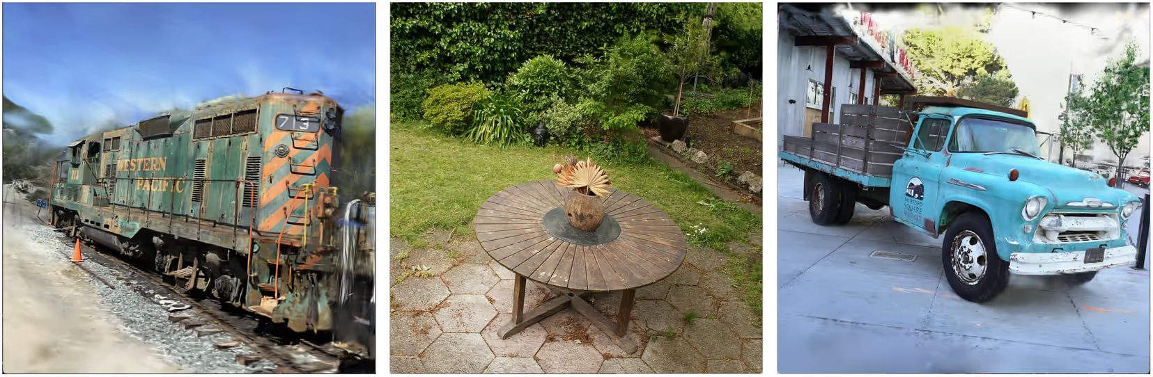
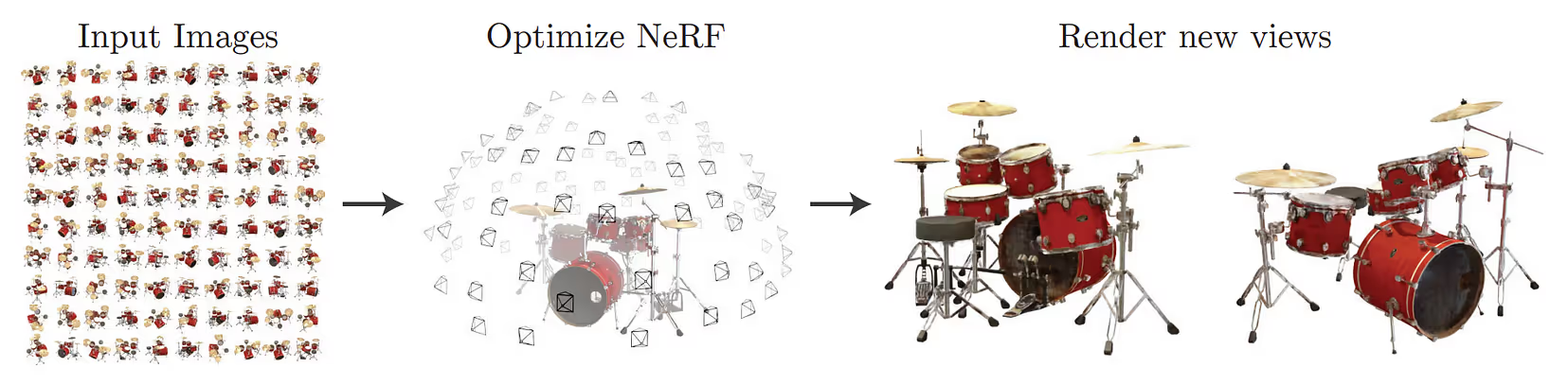
In recent years, 3D scanning and rendering have been the focus of significant research, leading to innovative developments. One such breakthrough in this field is the development of Neural Radiance Field methods, which have revolutionized novel-view synthesis in computer graphics by producing highly detailed and photorealistic renderings.
Traditional photogrammetry often struggles with varying lighting conditions and capturing fine details. NeRF models attempt to alleviate these issues by utilizing a neural network to represent the scene’s radiance and density. The process involves training the neural network (the radiance field) to match a set of input 2D images by sampling the network’s output through ray marching and minimizing the difference between the input views and the rendered images.
However, NeRF is computationally demanding, as the process of training a NeRF model and rendering views is resource-intensive, often requiring significant processing time and power.
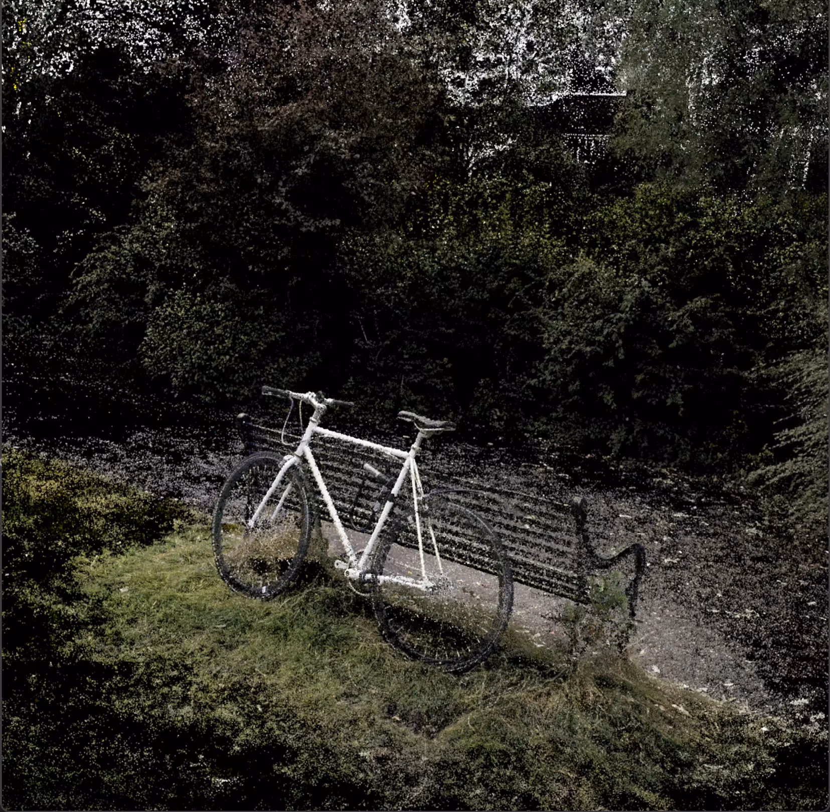
3D Gaussian Splatting, originally introduced in the paper 3D Gaussian Splatting for Real-Time Radiance Field Rendering, tries to address these issues by using 3D Gaussians to represent the scene. This method approximates volume rendering by projecting (or “splatting”) the Gaussians and blending the results, rather than marching rays through the scene. In contrast to Neural Radiance Fields, this approach optimizes a set of Gaussians rather than a neural network and utilizes rasterization, allowing for significantly faster rendering compared to ray marching. However, compared to NeRF, the storage requirements are significantly higher, which still poses challenges for practical deployment.
Representing a scene with Gaussians
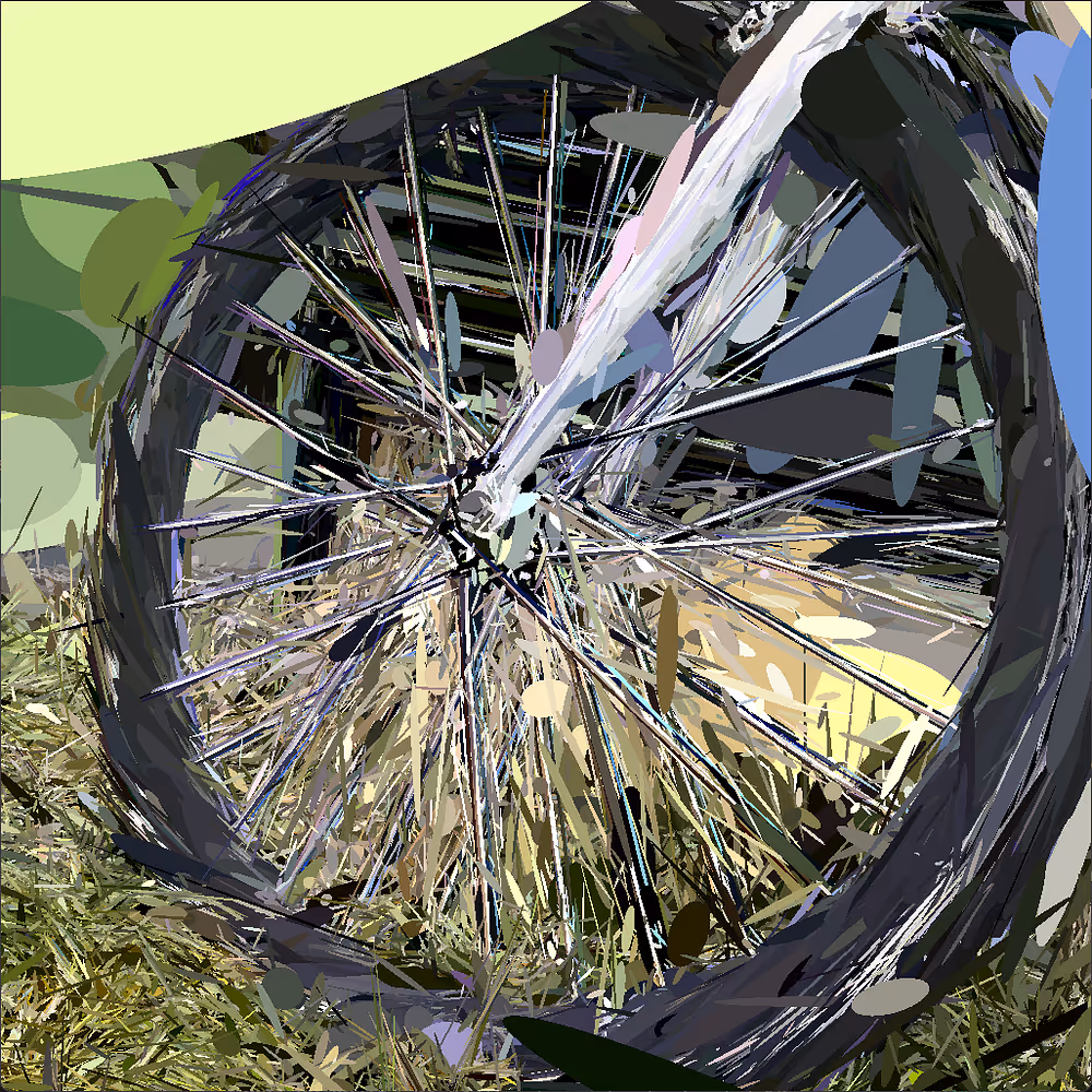
In Gaussian Splatting, a 3D scene is represented by a set of points, each corresponding to a 3D Gaussian. Unlike NeRF, where the scene is modeled using a neural network, Gaussian Splatting represents the scene directly with these 3D Gaussians.
Each Gaussian is fitted with a unique set of parameters so that the rendered images match the known dataset. The parameters of each Gaussian include:
- Mean (or position), which defines the center of the 3D Gaussian
- Covariance matrix, which determines scale and rotation of the Gaussian
- Opacity
- Color — either RGB values or spherical harmonics coefficients


Implementing the 3D Gaussian Splatting Rendering Algorithm
Now that we understand Gaussians and how to represent a scene with them, we can delve into the practical implementation of the rendering algorithm suggested in the original paper. Although it is possible to use the standard rasterization pipeline for rendering Gaussians, using compute shaders with tile-based rasterization offers finer control over GPU resources used and can enhance performance through fast GPU sorting algorithms for alpha blending.
For context, in this example, I’ll use the Breda framework, which supports render graphs, bindless resources, and HLSL shader code (compiled for DX12, Vulkan and Metal backends). However, the logic and structure of this rendering algorithm can be adapted to any modern rendering API.
Method Overview:
- Split the Screen into Tiles: Divide the screen into a grid of tiles (e.g., 16x16 pixels).
- Pre-process Gaussians: Transform Gaussians into screen space, calculate how many tiles each Gaussian occupies, and compute their color and depth from the camera’s point of view.
- Create Keys for Each Gaussian Instance: Duplicate Gaussians that occupy more than one tile and assign keys (containing tile ID and depth) to each instance.
- Sort Keys: Sort the keys based on the tile ID and the depth values of the Gaussians.
- Calculate Tile Workload Ranges: Determine the workload for each tile based on sorted keys.
- Render Tiles: Use the sorted data to render each tile efficiently.
Since this blog post focuses on the rendering part, we can use pre-trained models provided by the original paper’s authors. These models, stored as .ply files, include all parameters for each Gaussian. After extracting the necessary data from the file, we start rendering by first splitting the screen into tiles. For now this part doesn’t require any code, so we can proceed to the pre-processing step to prepare Gaussians for rendering.
Pre-processing Step
The pre-processing step involves transforming Gaussians into screen space, determining the number of tiles each Gaussian occupies, and computing the output color using spherical harmonics.
We start by creating a set of buffers from the data obtained from the .ply file, storing Gaussian parameters: positions, opacities, and spherical harmonics coefficients. If we choose to compute the 3D covariance matrix on the GPU, we store scale and rotation values; alternatively, we can precompute this matrix on the CPU and only send the upper half to the GPU, as the matrix is symmetric. This pre-processed data forms our input.
For the output, we store:
- Screen Space Position: The position of the Gaussian in screen space.
- Depth: Depth information for each Gaussian.
- Radius: The projected 2D radius of each Gaussian.
- RGB Color: Calculated from spherical harmonics.
- Conic Section: Stores a 3D vector defining the splatted Gaussian; we can additionally pack it with the original opacity obtained from the file.
- Tile Count: Stores how many tiles each Gaussian occupies.
Within the Breda framework, creating these buffers and using the compute shader pipeline is especially straightforward. The framework’s abstractions remove the need for users to have specific knowledge of the underlying rendering APIs, ensuring compatibility across Vulkan, DX12 and Metal, allowing to focus on developing the algorithms and logic.
1// Create static buffers for pre-process input
2let positions = render_graph_persistent_store.create_static_buffer_with_data(
3	"gaussian positions",
4	&BufferCreateDesc::gpu_only_constants(),
5	&gaussian_data.positions,
6);
7
8// Create storage buffers for pre-process output
9let point_image_buffer = render_graph.create_storage_buffer(
10	"point image out buffer",
11	gaussian_bindings.num_of_gaussians * std::mem::size_of::<f32>() * 2,
12);
13
14// Pre-processing the gaussians
15// Involves transforming them into screen space,
16// determining the number of tiles each Gaussian occupies and
17// computing the output color from spherical harmonics
18ComputePass::new("Preprocess Gaussians", render_graph)
19    .constant(viewer_constants)
20    .read(&gaussian_bindings.positions)
21    .read(&gaussian_bindings.scales)
22    .read(&gaussian_bindings.opacities)
23    .read(&gaussian_bindings.rotations)
24    .read(&gaussian_bindings.cov_3d)
25    .read(&gaussian_bindings.sh)
26    .write(&point_image_buffer)
27    .write(&depth_buffer)
28    .write(&radii_buffer)
29    .write(&rgb_buffer)
30    .write(&conic_opacity_buffer)
31    .write(&tiles_buffer)
32    .dispatch(
33        &shader_db.get_pipeline("preprocess-gaussians"),
34        gaussian_bindings.num_of_gaussians.div_ceil(GROUP_SIZE) as u32,
35        1,
36        1,
37    );
In the pre-processing shader, we first check if the mean (position) of the Gaussian is within the view frustum. If it is, we proceed to compute the covariance in 2D, from which we can derive the conic section and radius of the Gaussian:
1float3 cov = computeCov2D(mean, focalX, focalY,
2                          tanFovX, tanFovY, cov3D, worldToView);
3
4float det = (cov.x * cov.z - cov.y * cov.y);
5if (det == 0.0f)
6    return;
7
8float det_inv = 1.f / det;
9float3 conic = {cov.z * det_inv, -cov.y * det_inv, cov.x * det_inv};
10
11float mid = 0.5f * (cov.x + cov.z);
12float lambda1 = mid + sqrt(max(0.1f, mid * mid - det));
13float lambda2 = mid - sqrt(max(0.1f, mid * mid - det));
14float radius = ceil(3.f * sqrt(max(lambda1, lambda2)));
The computation of the covariance matrix in 2D follows the steps outlined in equations 29 and 31 of the “EWA Splatting” method (Zwicker et al., 2002), with modifications to account for screen size and aspect ratio (as used in the the original paper).
Calculating the screen space coordinates and depth is straightforward. However, we still need to determine how many screen-space tiles each Gaussian occupies. To do this, we compute the area of the axis-aligned bounding box (AABB) that the projected Gaussian covers in 2D. Knowing the area of the tiles allows us to calculate the number of tiles a Gaussian occupies.
1uint2 tileGrid = uint2((bnd.constants.resolution.x + kBlockX - 1) / kBlockX,
2                      (bnd.constants.resolution.y + kBlockY - 1) / kBlockY);
3getRectFromRadius(pointImage, radius, rectMin, rectMax, tileGrid);
4
5uint tilesTouched = (rectMax.x - rectMin.x) * (rectMax.y - rectMin.y);
6
7// Quit if processed Gaussian occupies 0 tiles
8if (tilesTouched == 0)
9    return;
The final task in the pre-processing step is to compute the color. This can be done using either RGB values or spherical harmonics. Spherical harmonics (often referred to as SH) are particularly useful for encoding colors in a view-dependent manner, which improves the quality of renders by allowing the model to represent non-Lambertian effects, such as the specularity of metallic surfaces.

Key Generation and Sorting
Next, we compute the inclusive sum of the buffer containing the number of occupied tiles. For example, if the input buffer is [0, 2, 0, 1, 3], the output buffer would be [0, 2, 2, 3, 6], representing the cumulative sum. To achieve this, we implement a parallel prefix sum algorithm. While this implementation, sourced from Unity forums, may not be the most efficient, it is well-suited for Gaussian Splatting and compatible with HLSL code. The resulting output buffer provides the offsets necessary for generating keys and determining the total number of Gaussian instances to render.
With the number of Gaussians to render known, we allocate buffers for keys and values. The paper suggests using a 64-bit value for keys, combining both depth and tile ID, which allows efficient sorting. During key generation, we iterate through each tile occupied by a Gaussian, writing entries into the key and value buffers based on the offsets from the previous step.
1[numthreads(256, 1, 1)] void main(uint threadId : SV_DispatchThreadID) {
2    BufferBindings bnd = loadBindings<BufferBindings>();
3    uint idx = threadId;
4
5    if (idx >= bnd.constants.gaussianNum)
6        return;
7
8    uint3 tileGrid = uint3((bnd.constants.resolution.x + kBlockX - 1) / kBlockX,
9                           (bnd.constants.resolution.y + kBlockY - 1) / kBlockY, 1);
10    int radius = bnd.radii.loadUniform<int>(idx);
11
12    if (radius > 0) {
13        uint offset = (idx == 0) ? 0 : bnd.offsets.loadUniform<uint>(idx - 1);
14
15        uint2 rectMin, rectMax;
16
17        float2 xy = bnd.pointImage.loadUniform<float2>(idx);
18        float depth = bnd.depth.loadUniform<float>(idx);
19
20        getRectFromRadius(xy, radius, rectMin, rectMax, tileGrid);
21
22        for (int y = rectMin.y; y < rectMax.y; y++) {
23            for (int x = rectMin.x; x < rectMax.x; x++) {
24                DuplicateKey key = (DuplicateKey)0;
25                key.tileId = uint(y * tileGrid.x + x);
26                key.depth = depth;
27
28                bnd.gaussianKeys.store<DuplicateKey>(offset, key);
29                bnd.gaussianValues.store<uint>(offset, idx);
30                offset++;
31            }
32        }
33    }
34}
Once keys are generated, we sort them. The Breda framework provides GPU sorting algorithms such as FFX and OneSweep, which were straightforward to use.
Tile Workload Calculation
With a sorted list of Gaussian keys and values, we compute the workload for each tile. This step eliminates the need to check for workloads in the rendering shader. By checking where in the sorted list of keys tile ID changes, and by storing thread ID, we create a buffer that defines workload ranges for each tile for rendering.
Rasterization
For rasterization, we launch one thread block per 16x16 pixel tile. Each dispatch processes one tile by loading packets of Gaussians into shared memory. For each pixel in the tile, we accumulate color and alpha (α) values (blending is based on the initial sorting). When the target saturation α is reached in a pixel, the corresponding thread stops, and the output is written into the render target.
Conclusion
There are still a few opportunities to improve Gaussian Splats rendering, such as optimizing the size of the structures used, explored by Aras Pranckevičius in his blog post, or issues related to approximation in both training and rendering, addressed in the following research.
As an intern, I gained valuable experience and enjoyed working with a talented and supportive team at Traverse Research. The environment in the company made it easy to seek help when needed. The codebase, with its efficient implementation and clear abstractions of common algorithms like sorting, was a pleasure to work with.