
Learning About GPUs Through Measuring Memory Bandwidth
At Traverse Research, we need to have a deep understanding of GPU performance to develop our benchmark, Evolve. Additionally, we sometimes do projects for very specific hardware where we need to know all the ins and outs of this hardware. One way we do this is by using microbenchmarks to measure specific parts of the GPU to get new insights. In this article, we will share what we learned from measuring the memory bandwidth of various GPUs. First we will be going over some background information about GPU hardware relating to loading from and storing to memory, then we will take a look at how our microbench is built, and finally we will look at some GPUs of which we measured the bandwidth and what we learned from that.
Background Information
Accessing memory on a GPU is quite a bit more complicated than on a CPU. In this section we will talk about different concepts that are handy to keep in mind when programming for a GPU.
Descriptors
Memory on a GPU is usually not directly accessed via a pointer like on a CPU. Although some hardware is capable of doing this, buffer and textures access usually happens via a descriptor. A descriptor is nothing more than a pointer with extra metadata to support more complex logic when fetching data. For example for a texture the hardware needs to know the resolution, swizzle pattern, format, number of mip levels, whether the texture uses MSAA, and more to be able to load from it. This is all encoded in the descriptor. How this descriptor is represented in binary is up to the hardware vendor and is thus something we generally cannot see directly. Buffers are also accessed via a descriptor but often only encode a pointer with a size. If you ever wondered how the hardware is able to return a default value when reading out of bounds, this is how.
Types of buffers
When talking about buffers there are a couple of distinctions we need to make between the various sorts, since each have their own advantages and disadvantages.
1. Byte Address Buffers
The most basic form is a Byte Address Buffer, or sometimes called the Raw Buffer, this type allows us to load any data type in the shader by passing a byte offset. However, that is not the complete story. GPUs are generally not able to access non-4-byte aligned data, so the byte offset in reality has to be a multiple of 4. Additionally, most hardware is able to load in data in chunks of 4, 8 and 16 bytes. This reduces the number of load requests. Some hardware is able to load these larger chunks from any 4-byte aligned address, but not all hardware is able to do so. Since Byte Address Buffers do not give any guarantees in terms of alignment the shader compiler may generate four 4-byte loads instead of a single 16-byte load.
2. Structured Buffers
Structured Buffers are a more strict version of the Byte Address Buffer. The graphics API requires the user to specify the size of the data type. Additionally, when not using bindless, a StructuredBuffer in the shader can only load one data type. These restrictions allow the driver and shader compiler to guarantee that data is aligned in an optimal way to allow for 8 and 16-byte load instructions.
3. Typed Buffers
Typed buffers are a bit more special as they use some of the functionality of the texture units. This allows us to load from, for example, a RGBA8_UNORM buffer and let the hardware unpack it to a float4. If we were to use for example a raw buffer, we would need to use ALU instruction to do this conversion. Of course this is a nice advantage but using the texture units is not always free either. The general advice is to not use typed buffers unless you really need the extra ALU that would otherwise have been spent the data unpacking.
Texture Units
While buffer loads are fairly straightforward, texture loads can get quite complicated. What's interesting is that all this extra complexity can be implemented partially or entirely in software, but it is often implemented in hardware for performance. Although this bit of the hardware comes in many flavors, we tend to refer to this bit of the hardware as the 'texture units'.
Let's go through the complexities that the texture units do one step at a time. Firstly, a texture load can be 1D, 2D, 3D, have mip levels, be an array, be a cubemap, or a mix of these. For each of these formats a floating point coordinate needs to be converted to a texel coordinate. Secondly, there are the address mode sampler settings that decide whether UV coordinates need to be wrapped around, clamped, mirrored or if a border color needs to be used. Finally, the filtering mode also has an impact on the address calculation, as with linear and anisotropic filtering, more than one texel needs to be loaded. All this together can result in a lot of logic and texel loads, just imagine doing an anisotropic sample in the corner of a cubemap array texture.
The texture units do more than only address calculation. When it loads a texel, it may also need to unpack it to a float32 value. For a format like RGBA8_UNORM this is four relatively simple byte to float conversions, but the format may also require an sRGB calculation or use a more complicated block compressed format. To give an example of such a format, in the block compressed formats of PC GPUs, BC1 till BC3, we find two 16-bit colors with a 4x4 matrix of 2-bit elements. Each element indicates how to blend the two 16-bit colors together to create the decompressed color. Finally, the texture unit blend all the loaded texels together which is then stored in the requested register for use by the shader.
Memory Hierarchy
Due to physical limitations like the speed of light it is impossible to have a large amount of VRAM like 16GiB be fast enough to keep up with the computational speed of a GPU. This is both a limitation in bandwidth and latency. To alleviate this problem caches are added in various places in the chip. These vary in size and speed as well as proximity to where ALU operations happen. The general rule of thumb is, the closer a cache is to where computation is happening, the faster and smaller it is. On most hardware we find at least 2 levels of cache (L1 and L2) as well as an instruction cache (I-Cache). AMD's RDNA4 hardware even has an L0, L1, L2, Infinity Cache, Instruction Cache, and Scalar Cache. The multiple levels of cache complement each other to create a good balance between size and performance.
Write-through vs write-back vs write-around
Caches do impose an interesting problem when it comes to writing data, do you let the write go through the other caches to main memory, do you wait until the cache line is evicted, or do you skip the cache entirely? These different approaches are called 'write-through', 'write-back', and 'write-around'. In general, we mostly find the write-back approach on GPUs. The advantage of this approach is something called 'write combining'. This lets more stores accumulate on the same cache line so that the whole line can be written into the next level of the memory hierarchy all at once when the cache line is evicted instead of a small store every time a store happens.
The caches in a GPU are really optimized for this type of spatially local memory access, where these bursts of memory can be read or written at the same time. When a shader accesses data in a very sparse pattern, the hardware can try to coalesce these memory requests where possible, but will at some point have to send out more requests than if the memory accesses were more spatially local.
Some algorithms may require reading data generated by other threads in the same shader. A simple example of this is a BVH refit where you have a thread per node. Each thread traverses up the tree and would start working on the same data as its neighboring thread, except that we use atomics to kill the thread that got there first. That creates the guarantee that one thread is working on one node. What now needs to happen is that the thread needs to load the AABBs of the child node. However, one of these child node AABBs may been generated by a thread on the other side of the machine, and may still be stuck in an L1 cache we cannot access. To overcome this the 'globallycoherent' keyword can be used. This keyword indicates that writes should be done using some kind of write-through or write-around method until the first cache that is accessible for all the cores on the GPU. This guarantees that even though the data was written by a core that doesn't share the same L1 cache, we can still read it from L2.
Hiding Latency
Even with caches, there will still be situations where data is not in cache and has to be fetched from main memory. To deal with this, the GPU can hold more threads in flight than it can execute at once. Instead of letting a compute unit idle, it just switches to a different wave of threads to execute while it waits for the memory request to finish. By letting a shader not use too many registers or groupshared memory, a compute unit can keep many of them in flight, increasing the chance of not idling.
It is important to note though that having more waves of threads in flight on the GPU is not always better for performance. In either very ALU or memory bandwidth-intensive use cases it can cause cache trashing because the relatively small cache cannot absorb all the memory accesses from all the waves. To illustrate this, imagine a cache line getting loaded in, and by the time it is accessed again, it has already been evicted from the cache due to so many other memory accesses of other cache lines causing it to get evicted. If fewer waves are running at a time the cache line may not have been evicted by the memory accesses of another wave.


Designing a Microbenchmark
A bandwidth microbenchmark can be as simple as creating a large buffer, running a shader, and reading every value from it. The read value has to be used in some way, otherwise the compiler will optimize the read out. The easiest way to do this is simply to write the value to a buffer.
1// Version 1
2[numthreads(256, 1, 1)]
3void main(uint dispatchThreadId: SV_DispatchThreadID) {
4    float4 value = inputBuffer.load(dispatchThreadId);
5    outputBuffer.store(dispatchThreadId, value);
6}
However, this is not quite a read bandwidth benchmark, since we are not only measuring the read, but also the write. Luckily, there are two things we can do to improve. First of we can write our data into a very small buffer so that it fits in our nearest cache. That will turn the shader into this.
1// Version 2, write to tiny buffer
2[numthreads(256, 1, 1)]
3void main(
4    uint dispatchThreadId: SV_DispatchThreadID,
5    uint groupThreadId: SV_GroupThreadID) {
6
7    float4 value = inputBuffer.load(dispatchThreadId);
8    outputBuffer.store(groupThreadId, value);
9}
Secondly, we can amortize the cost of all the overhead (like dispatching the shader, spawning threads, writing to memory, etc) by performing many reads using a loop. Additionally, we can unroll the loop to amortize the cost of the loop itself.
1// Version 3, amortize the overhead by performing many reads
2#define GROUP_SIZE 256
3[numthreads(GROUP_SIZE, 1, 1)]
4void main(
5    uint groupId: SV_GroupID,
6    uint groupThreadId: SV_GroupThreadID) {
7
8    uint groupLocation = groupId * GROUP_SIZE;
9    float4 acc = 0.0;
10
11    for (int i = 0; i < constants.loop; ++i) {
12        acc += inputBuffer.load(groupLocation + groupThreadId);
13        groupLocation += GROUP_SIZE;
14        groupLocation = (groupLocation == constants.valueCount) ? 0 : groupLocation;
15
16        acc += inputBuffer.load(groupLocation + groupThreadId);
17        groupLocation += GROUP_SIZE;
18        groupLocation = (groupLocation == constants.valueCount) ? 0 : groupLocation;
19
20        acc += inputBuffer.load(groupLocation + groupThreadId);
21        groupLocation += GROUP_SIZE;
22        groupLocation = (groupLocation == constants.valueCount) ? 0 : groupLocation;
23
24        acc += inputBuffer.load(groupLocation + groupThreadId);
25        groupLocation += GROUP_SIZE;
26        groupLocation = (groupLocation == constants.valueCount) ? 0 : groupLocation;
27    }
28
29    outputBuffer.store(groupThreadId, acc);
30}
Caches vs VRAM
The next problem we run into is that our measured read bandwidth of main memory is shooting through the roof. This is because we are reading data from the cache instead of VRAM! This is something we would also like to measure, but let’s first fix the VRAM measurement.
Avoiding constant cache hits is fairly simple. If we let every group start at a different part in the buffer, the chance that we are loading a chunk of memory that is in cache becomes nearly 0.
When measuring memory bandwidth, we need to take into account that there are various caches between the compute units and the main memory. Luckily, by measuring with increasingly larger buffers and carefully picking the location we load from, we can trigger as many cache misses as possible. When using a tiny buffer, we will practically be guaranteed to hit the nearest cache, and with a large buffer, like 1 GiB, we will always load from VRAM.
1// Version 4, Spread the groups to prevent cache hits
2#define GROUP_SIZE 256
3[numthreads(GROUP_SIZE, 1, 1)]
4void main(
5    uint groupId: SV_GroupID,
6    uint groupThreadId: SV_GroupThreadID) {
7
8    // On the CPU:
9    // uint bufferChunks = valueCount / (GROUP_SIZE * LOADS_PER_LOOP)
10    // uint chunkStride = (loopCount + bufferChunks + 1) * (GROUP_SIZE * LOADS_PER_LOOP);
11
12    uint groupLocation = (groupId * constants.chunkStride) % constants.valueCount;
13
14    float4 acc = 0.0;
15    for (int i = 0; i < constants.loop; ++i) {
16        acc += inputBuffer.load(groupLocation + groupThreadId);
17        groupLocation += GROUP_SIZE;
18        groupLocation = (groupLocation == constants.valueCount) ? 0 : groupLocation;
19
20        cc += inputBuffer.load(groupLocation + groupThreadId);
21        groupLocation += GROUP_SIZE;
22        groupLocation = (groupLocation == constants.valueCount) ? 0 : groupLocation;
23
24        acc += inputBuffer.load(groupLocation + groupThreadId);
25        groupLocation += GROUP_SIZE;
26        groupLocation = (groupLocation == constants.valueCount) ? 0 : groupLocation;
27
28        acc += inputBuffer.load(groupLocation + groupThreadId);
29        groupLocation += GROUP_SIZE;
30        groupLocation = (groupLocation == constants.valueCount) ? 0 : groupLocation;
31
32    }
33    outputBuffer.store(groupThreadId, acc);
34}
Another advantage of this version of the microbenchmark is that we can have any number of threads and any-sized buffer. This allows us to both test with many more threads than elements in the buffer to get a more stable timing, as well as use tiny buffers to measure the size and speed of the caches.
Textures vs Buffers
While at first sight, loading from a storage texture or a buffer seems like almost the same operation, they might be handled very differently in hardware. By testing both textures and buffers, we can find these differences. Additionally, we use a mix of buffers and textures to see if the given GPU has a ratio where bandwidth is highest.
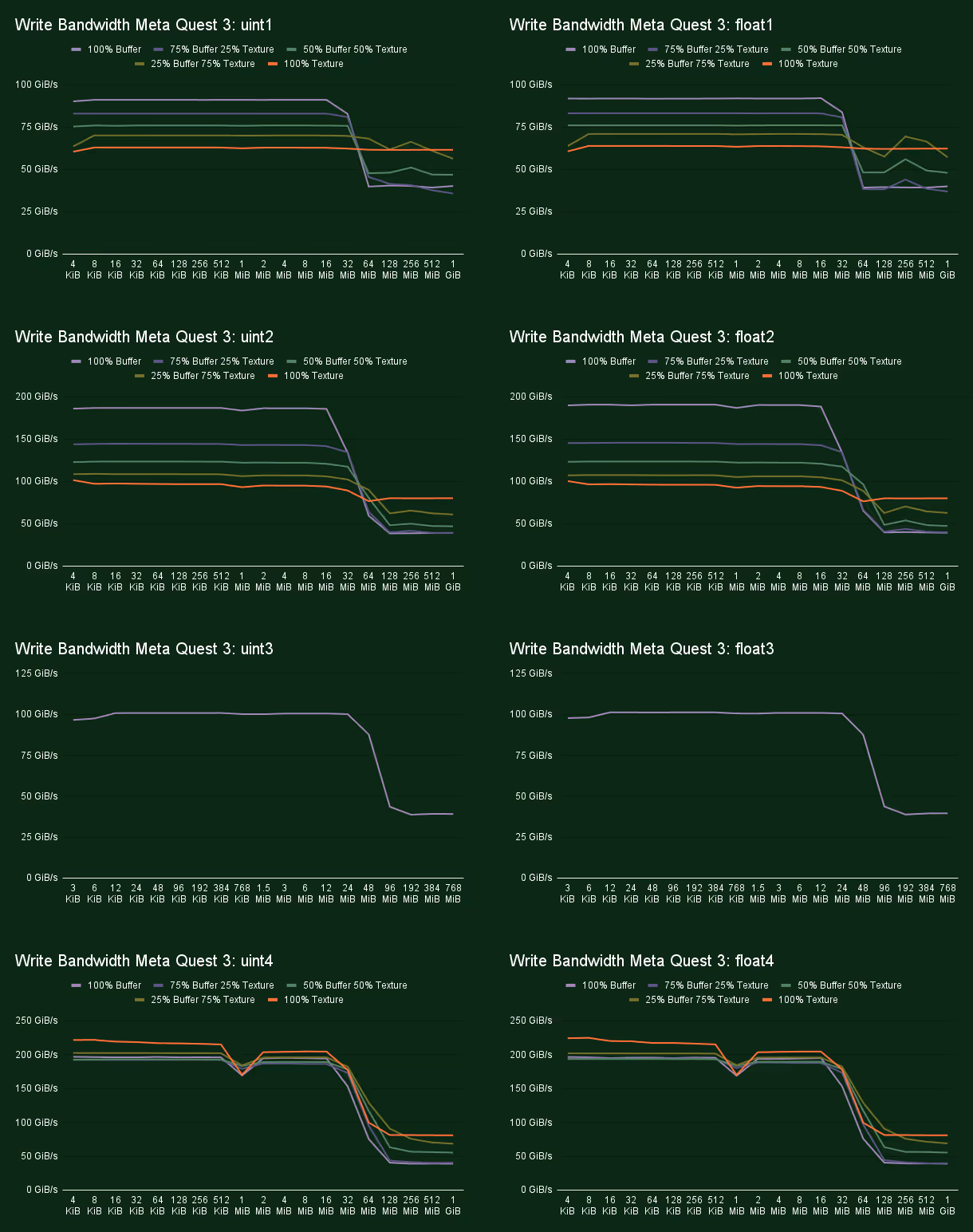
Stores vs Loads
Stores and loads can be handled quite differently in hardware, so this is an interesting thing for us to measure as well. Luckily, we need very few modifications to our benchmark to achieve this. We simply remove our dummy write at the end, replace all our reads with writes, and increment the accumulator by 1 every store to prevent the compiler from trying to optimize something we don’t want it to.
Element Formats
When loading and storing, we might be bottlenecked by the number of bytes that we can move over the memory bus, but can also be bottlenecked by the number of loads and stores we can issue. By using 4, 8, 12, and 16 byte element sizes, we can find these limitations. We implemented this in the shader using a simple macro for the data type.

Findings
Running the microbenchmarks on various hardware has been very insightful. From learning various quirks in different chips, to finding surprising bottlenecks in our microbenchmark.
IMPORTANT NOTE: These benchmarks are not comparisons as to which GPU is ‘better’. They are just measurements to learn about the different GPU architectures. For this reason, we have opted to use GPUs from different price brackets and power targets. We are not interested in ‘this number is higher on this GPU’, but more interested in what patterns are slow or fast on a given piece of hardware. If you are interested in comparing the real-world performance of GPUs, the Evolve benchmark suite is great for this!
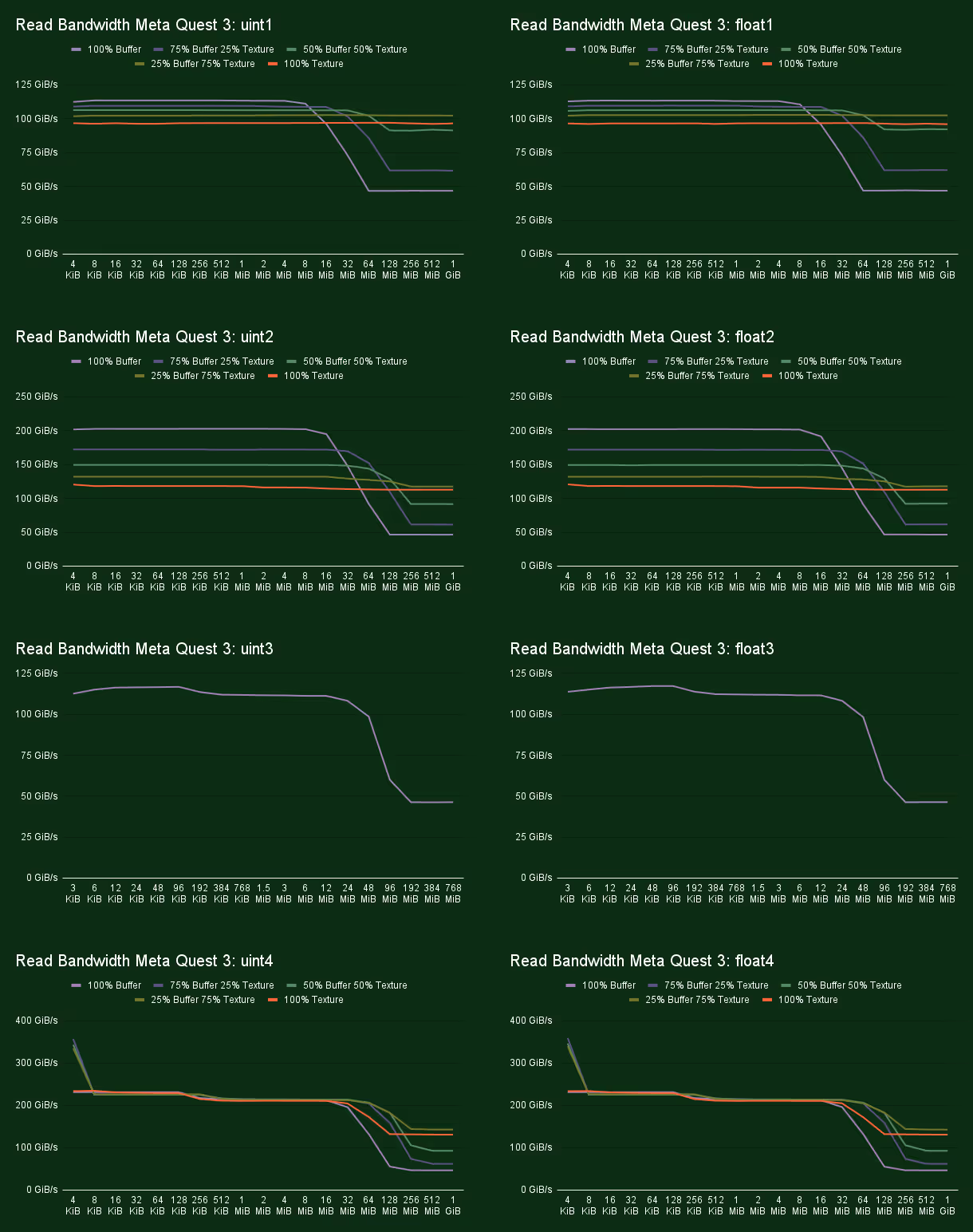
Qualcomm Adreno 740 (Meta Quest 3)
Let’s start off with a mobile chip, the Qualcomm Adreno 740 in the Meta Quest 3. This GPU has 12 Shader Processors, which each consist of 2 micro Shader Processors. We find a block of 1 KiB L1 cache per micro Shader Processor. Additionally, there is a block of shared L2 cache, and then further on a system level cache, which is usually shared with the CPU. From our measurements we see drop offs in read bandwidth after 128 KiB, 1MiB, and 8 MiB. For the write bandwidth we see clear drop off in performance at 512 KiB, but further drop offs after that are not quite as clear.
Other than differences in bandwidth between the caches we found some interesting data about using buffers vs textures. We found it to be fairly common for there to be a difference in bandwidth for data in cache across many GPUs. However, on the Quest 3 we found a significant bandwidth difference in main memory. It is significant enough that, when designing software specifically for this hardware, it would be worth it to replace large buffers with textures to achieve a near 3x bandwidth improvement from around 46 GiB/s to over 130 GiB/s.
Also interesting to note is that we hit the highest VRAM bandwidth of 143 GiB/s when we mix in 25% buffer loads. Additionally, we can see that using buffers is fine as long as we manage to hit the cache. When writing code we would recommend to use whichever resource type is most natural, but when optimizing for the Meta Quest 3 you might want to replace specific large buffers with textures to get that higher bandwidth.
Finally it has to be noted that the memory bandwidth of the Adreno 740 on the Quest 3 is much lower than the other GPUs we tested for this article. This is because this GPU is designed for a much lower power budget. Increasing the memory bandwidth is definitely possible but not without sacrificing battery life. Instead Qualcomm, like other mobile GPU vendors, uses techniques like tile based rendering to reach good performance while minimizing memory traffic.
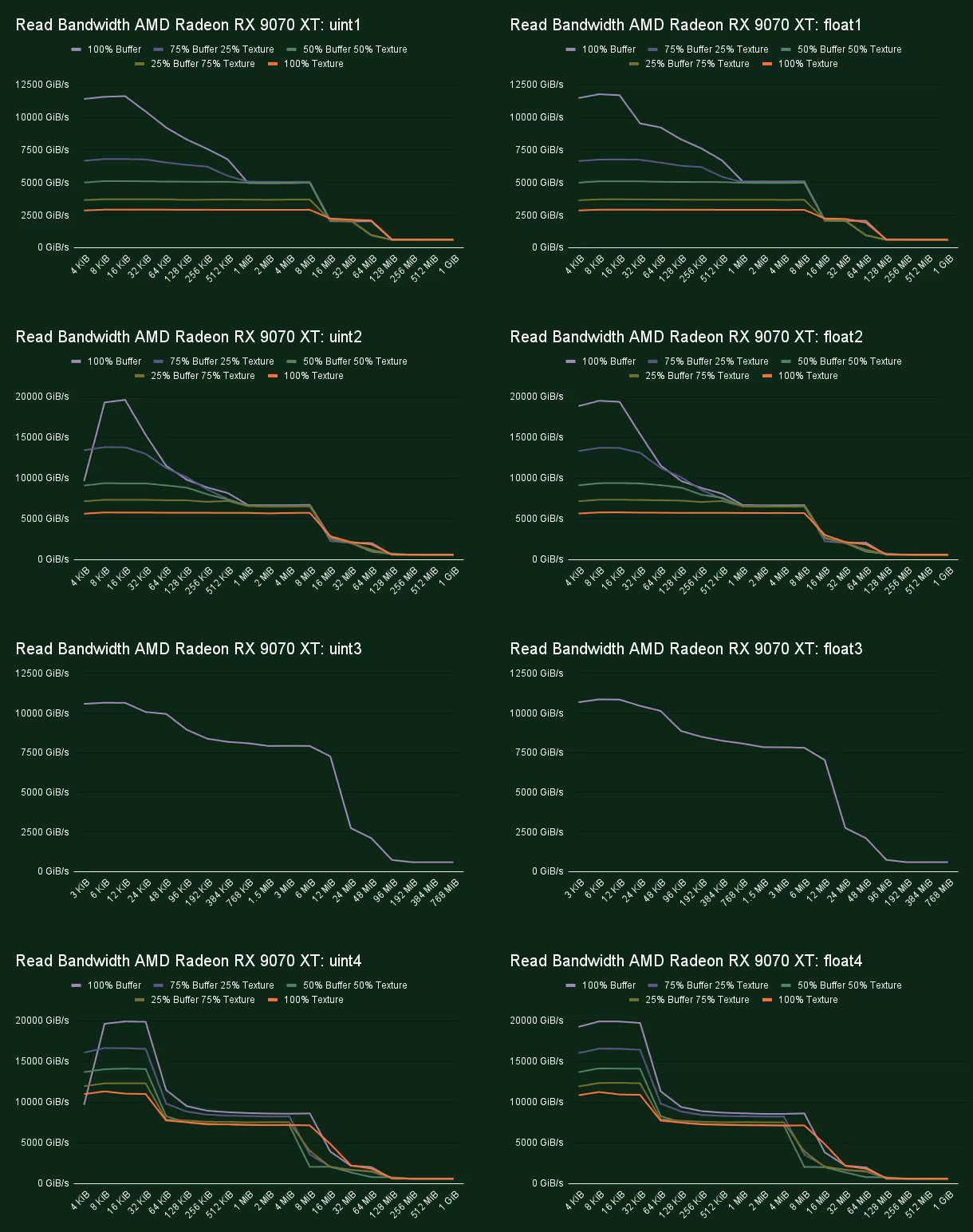
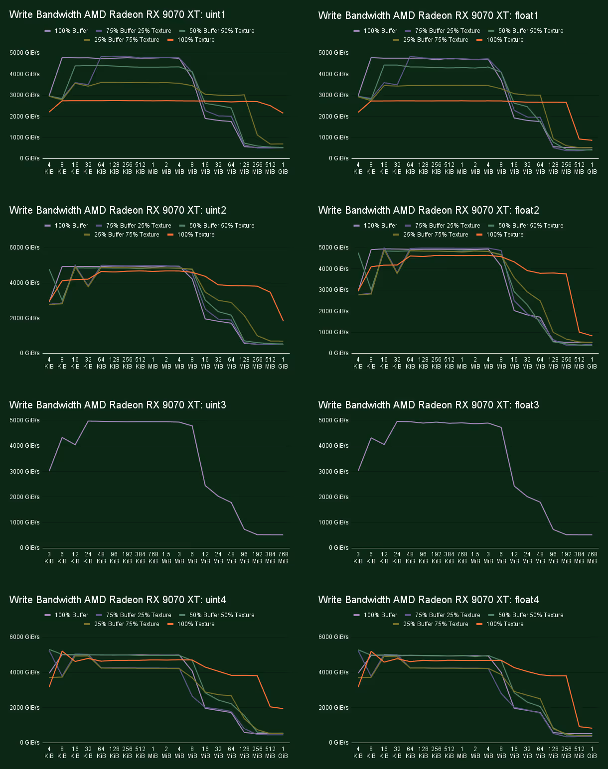
AMD Radeon RX 9070 XT
AMD has excellent documentation on what their hardware looks like. With the introduction of the RDNA architecture they released a white paper detailing the major differences, as well as releasing slides with what is new with each new iteration of their architecture. On top of that we also get a fully documented ISA full of little hardware details.
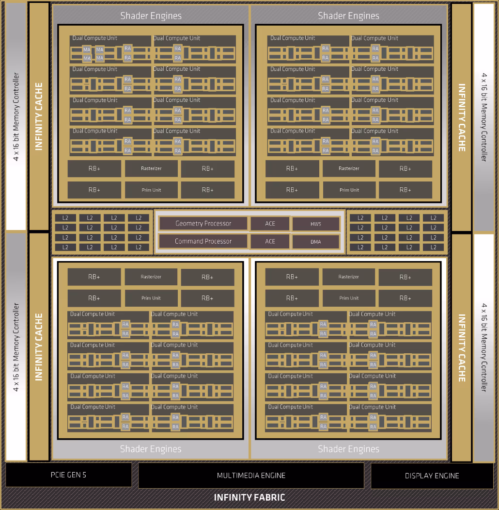
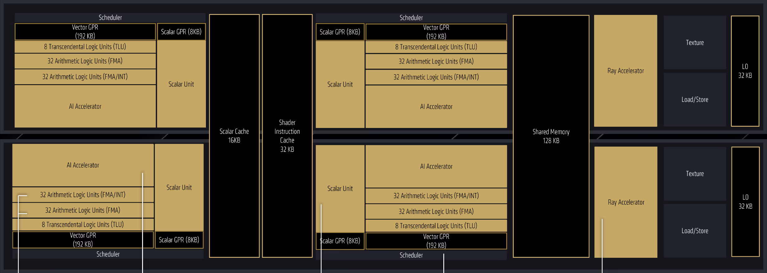
An AMD RDNA 4 GPU is built out of a various number of Shader Engines. Each Shader Engine consists of two Shader Arrays, and each Shader Array contains some Work Group Processors. In the case of the Radeon RX 9070 XT there are a total of 4 Shader Engines with 4 Work Group Processors per Shader Array. The Work Group Processor consists of 4 SIMDs divided into two Dual Compute Units. In a Work Group Processor we find 16KiB of scalar cache, 32 KiB of instruction cache, 128 KiB for groupshared memory, as well as two blocks of 32 KiB L0 cache, one for each Dual Compute Unit. Per Shader Array we find 256 KiB of L1 cache. This cache is also used for coherency gathering the load/store requests before moving on to the 8 MiB of L2 cache. Finally the RX 9070 XT has 64 MiB of infinity cache, which on RDNA 3 was on separate chiplets, but it is back on a monolith die in RDNA 4. The sizes of the caches can vary from GPU to GPU though, for example the Radeon RX 9060 XT has 4 MiB of L2 cache and 32 MiB of Infinity Cache.
When benchmarking the Radeon RX 9070 XT, we ran into an interesting problem. When measuring the bandwidth, we noticed a significant difference in performance when loading floating-point values vs integers. This had us quite confused since, from a hardware perspective, it should not matter whether you load an integer or a float.
It turns out we were running into an ALU bottleneck in our bandwidth benchmark! Just performing one integer multiplication per load was enough to be a bottleneck. When we replaced our dummy multiply op with an addition, we were able to measure the same bandwidth for both integer and floating point values.
I suppose we did not expect AMD’s L0 cache to be that fast. We managed to measure it at nearly 20 TiB/s when loading from a buffer. When loading from a storage texture, we only managed to reach 11 TiB/s.
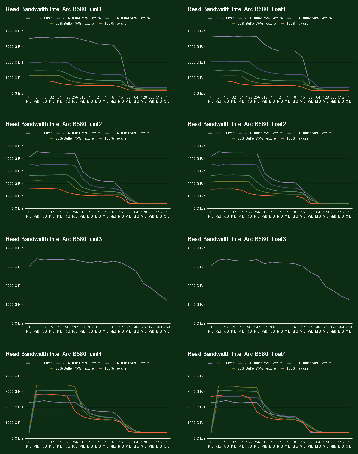
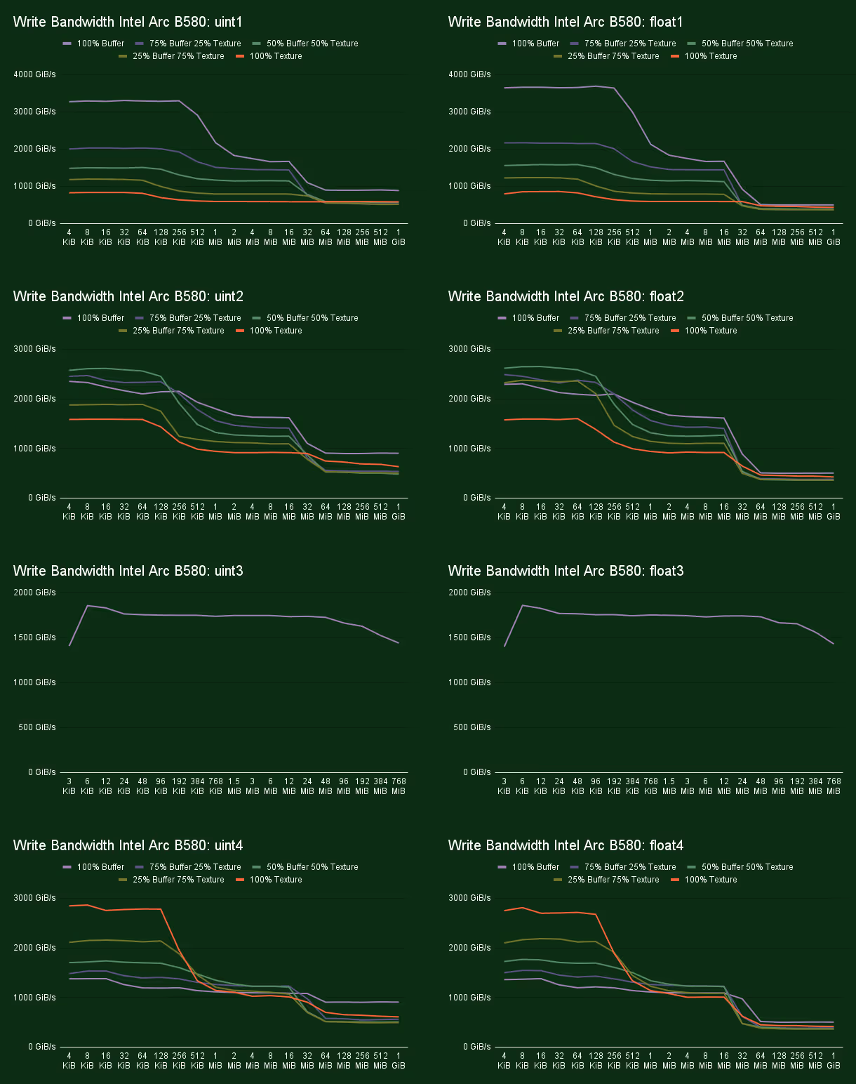
Intel Arc B580
Battlemage is Intel's second discrete GPU architecture. When it was announced with the introduction of the Intel Arc B580, they released some diagrams describing what their new GPU looks like under the hood, giving us some interesting insights.
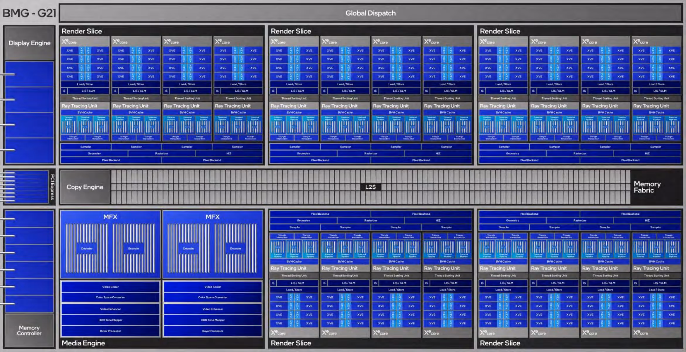
The Battlemage GPU architecture is built out of Render Slices, 5 in the case of the B580. Each Render Slice contains 4 Xe Cores as well as 4 Ray Tracing Units, 4 Samplers and some blocks for rasterization. Inside each Xe Core we find 8 Xe2 Vector Engines, 96 KiB of instruction cache and 256 KiB of L1 Cache. The L1 block is also used as groupshared memory where the block can be partitioned as needed. The main block of L2 cache is 18 MiB in size.
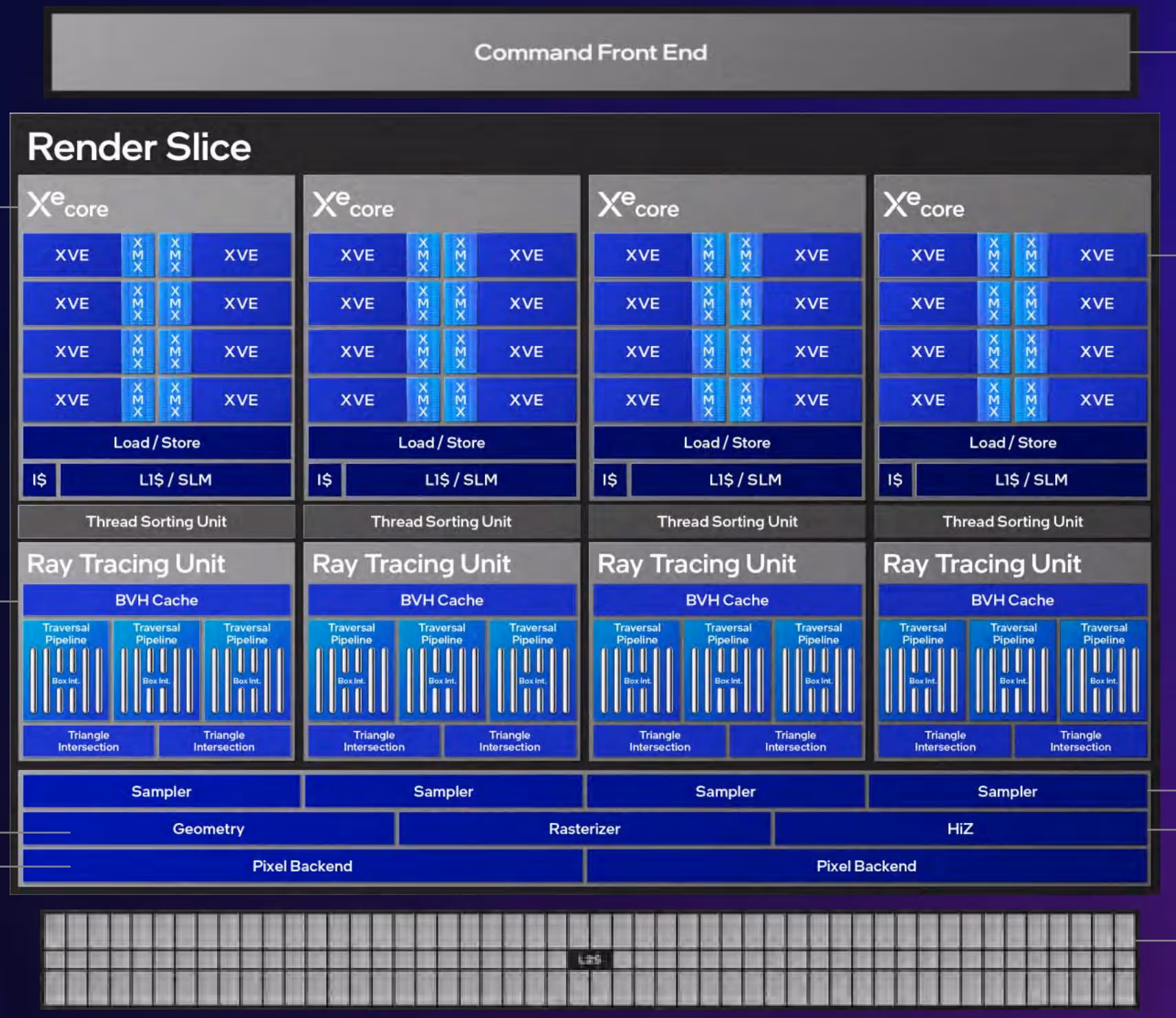
The B580 surprised us when comparing 4-byte vs 16-byte loads when loading from textures vs buffers. We found that for buffers, bandwidth goes down for larger data types, while for textures, it goes up for larger data types. This would suggest that data paths via buffers and textures, for the caches at least, seem to be optimized for different use cases.
A second interesting find is that bandwidth is lower for 12-byte elements. This is likely because it is being split into two separate memory transactions, limiting the bandwidth.
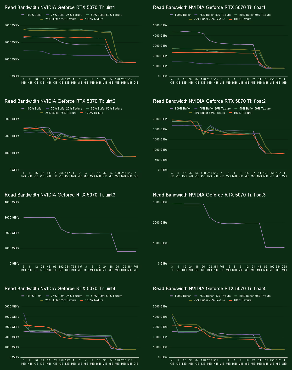
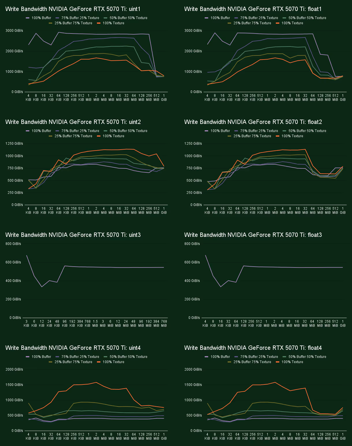
NVIDIA GeForce RTX 5070 Ti
NVIDIA's Blackwell architecture is by far the largest scaled of all all the current generation GPUs. When the new architecture was released they also released a white paper describing all the changes as well as some very useful diagrams. The diagram they released is of their full GB202 chip, of which a slightly cut down version is found in the GeForce RTX 5090, likely due to binning.
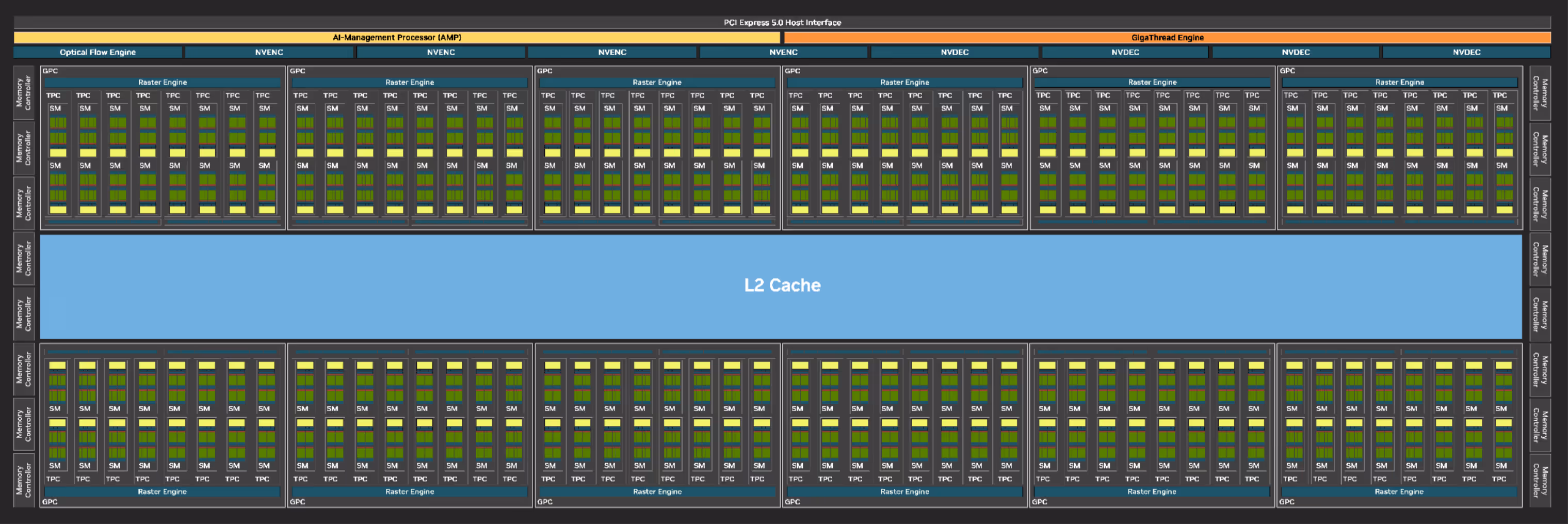
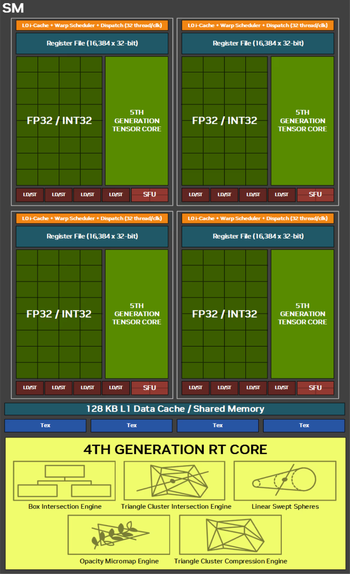
The NVIDIA GeForce RTX 5070 Ti we tested uses the same architecture but a smaller version of the chip. On chip we find 6 Graphics Processing Clusters (GPC), 35 Texture Processing Units (TPC), and 70 Shader Multiprocessors (SM). On the GPU we find 48 MiB of L2 cache, and as we zoom into the SM we find 128 KiB of L1 cache on each of them. The L1 block is also used for groupshared memory and can be split up with 10 different configurations ranging from 0 KiB to 228 KiB used for groupshared.
In benchmarking the RTX 5070 Ti we found that many writes to the same small piece of memory causes a large bottleneck reducing performance massively. To be fair, this is not a use case with any real world computation uses, but it's interesting to see and makes us wonder what exactly is happening in the hardware that causes this.
Another interesting find is that we saw a large decrease in read bandwidth when reading a uint1 from a buffer vs a float1. So far we found on AMD's Radeon RX 9070 XT that integer multiplies caused an ALU bottleneck. This case is different, as it's only the buffer loads that are affected, not the texture loads. We reran the microbench but got the same results back. So far we have not been able to explain why there is a difference in performance in this specific case.
Conclusion
With our new bandwidth microbenchmark we are just scratching the surface of what we can discover. So far we have been able to find that some paths can be faster on certain hardware like using textures vs buffers on the Meta Quest 3, or that loading 12-byte elements on Intel doesn't do well on the caches closest to the shader cores. However, we also found patterns that still remain a mystery to us. As we further develop our microbenchmarks we hope to uncover more insights on the hardware.
Generally, we don't let one pattern being slower or faster on one specific vendor affect the way we write code, as we don't want to favor one GPU vendor over another. However, the common patterns are certainly helpful. Additionally, for projects targeting specific hardware that are not Evolve related, this type of data can helps us to squeeze every bit of performance out.
We already have a lot of ideas for more microbenchmarks we want to build and try out. When we find some more interesting results we will share them with another blog posts so keep your eyes out for that!
Sources:
- https://chipsandcheese.com/p/inside-snapdragon-8-gen-1s-igpu-adreno-gets-big
- https://www.techpowerup.com/gpu-specs/radeon-rx-9070-xt.c4229
- https://www.amd.com/content/dam/amd/en/documents/radeon-tech-docs/instruction-set-architectures/rdna4-instruction-set-architecture.pdf
- https://www.techpowerup.com/review/amd-radeon-rx-9070-series-technical-deep-dive/3.html
- https://images.nvidia.com/aem-dam/Solutions/geforce/blackwell/nvidia-rtx-blackwell-gpu-architecture.pdf
- https://download.intel.com/newsroom/2024/client-computing/Intel-Arc-B580-B570-Media-Deck.pdf