Introduction

Hi everyone! In this blog post I will be detailing how we solved the problem of levels of detail for geometry and materials in our graphics framework Breda, which was needed for our next-gen benchmark Evolve. For this post I will focus on the more traditional solution that we went with, but we have also been experimenting with systems such as Nanite which you can read about here. Code samples are in Rust and HLSL.

‍

Why do we need LODs?

Evolve is a next-gen benchmark capable of measuring various aspects of your GPU to indicate how well it will perform in modern game-like workloads. As such, we need to closely mimic what games are doing and LODs are generally present in most engines in some form or another.

Another reason for LODs is the increased scene complexity in Evolve, which caused us to exceed our polygon budget for mobile hardware. LODs helped reduce the triangle count to meet our performance target for both ray-tracing and rasterization.

We also faced performance issues on mobile when most meshes in the scene had a specular layer, which in turn cause more rays to be traced and expensive ReSTIR Reflections passes to run. While expensive, the rough reflections at a distance were barely noticeable on low upscaled resolutions. LODs offered a solution here, as we could still keep the reflective layers when close to a mesh, while falling back to the cheaper to evaluate materials from afar.

The Asset Pipeline

The system starts offline when we define meshes in our workspace in various yaml files. Here we can specify the source assets for each LOD, as well as how much of the screen should be covered before transitioning. These files are automatically generated by a python script that exports our scenes from the editor as separate GLTF files.

scenes:
  mesh1:
    filename: "breda-storage://models/mesh1_LOD0.gltf"
    lods: ["breda-storage://models/mesh1_LOD0.gltf", "breda-storage://models/mesh1_LOD1.gltf", "breda-storage://models/mesh1_LOD2.gltf"]
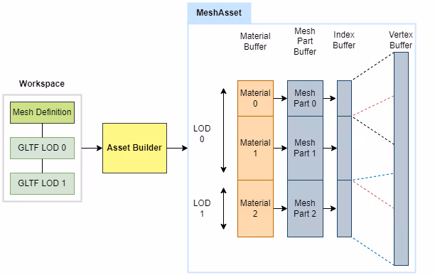
    lod_activation_screen_sizes: [1.000000, 0.800000, 0.400000]

The source assets are loaded into our asset building pipeline, where we convert them into MeshAssets which we cache. During this process, we build a single vertex and index buffer from all source LODs of a mesh. We also store metadata such as how many LODs there are and how many Mesh Parts there are per LOD. A Mesh Part in this case is a sub-set of vertices covered by a single material, defined by a range in the index buffer. Materials are mapped to their mesh part, and stored as a MaterialBatchAsset.

During this process, we automatically de-duplicate assets by checking their deterministic hashes. For example, two GLTF files specifying the same texture will result in only a single texture being processed and used at runtime.

During development, I added automatic LOD generation using an existing crate that culls the index buffer without touching the vertices. This was a quick solution for early testing and profiling while art was not yet ready, but did not result in high quality LODs suitable for release.

Runtime

Data Access

At runtime, we load the MeshAssets from disk. The next step is to make the data available on the GPU. Fortunately we use bindless rendering, which greatly simplifies this step.

First, we upload the Index Buffer and Vertex Buffer to the GPU. Next, we upload the Mesh Parts to a persistent GPU buffer that contains all mesh parts of all meshes. I made a freelist-allocator for GPU buffers for this purpose. We have to remember the offset in the Mesh Parts Buffer for each mesh, and also where each LOD starts and ends in that buffer. We also upload the materials to a monolithic buffer, of which the indices map 1:1 with the Mesh Parts Buffer.

// A mesh part is just an offset and size in the index buffer.
struct MeshPart {
  index_buffer_offset: u32,
  num_indices: u32,
}

// CPU sided tracking of data for a mesh.
struct CpuMeshData {
  vertex_buffer: Arc<dyn Buffer>,
  index_buffer: Arc<dyn Buffer>,
  mesh_part_buffer_offset: u32,

  num_mesh_parts_per_lod: Vec<u32>,
  mesh_part_offsets_per_lod: Vec<u32>,
  mesh_parts: Vec<MeshPart>,
}

Now we do some bookkeeping by creating buffers that map the unique identifier (NodeHandle) for each mesh instance in the scene to their vertex buffers, chosen LOD and mesh parts for each LOD. These bookkeeping buffers are stored in structs such as MaterialBindings and MeshBindings which we bind when we dispatch GPU work.

I will explain later how we choose the LODs, but for now just assume that for each node in the scene that has a mesh attached, we have chosen the appropriate LOD.

This is what indexing looks like in a pixel shader (pseudo-code):

struct Bindings { ... };

struct GpuMeshData {
    RawBuffer indexBuffer;
    RawBuffer positionsBuffer;
};

MainPS(uint triangleId : SV_PrimitiveID) {
  // Our bindless entrypoint.
  Bindings bnd = loadBindings<Bindings>();

  // The index of the mesh part we're rasterizing, can be a push constant.
  // This mesh part already is of a specific LOD.
  uint meshPartIndex;
  // The handle of the instance of the mesh we're drawing, push constant.
  uint nodeHandle;

  // Materials map 1:1 with mesh parts, so we can load it straight away!
  Material material = bnd.materialBindings.loadMaterial(meshPartIndex);
  
  // We keep a mapping between mesh instance and mesh data buffer index.
  // This gives us access to the index buffer and vertex buffer.
  // In a vertex shader, we could load the index and vertex.
  GpuMeshData meshData = bnd.meshBindings.loadMeshData(nodeHandle);

  // In rasterization we know the mesh part we're drawing,
  // We can index into a buffer to retrieve the index offset and size.
  // By this point, we can load the triangle specific data.
  MeshPart meshPart = bnd.meshBindings.loadMeshPart(globalMeshPartIdx);
  Triangle tri = meshData.loadTriangle(meshPart, bary, triangleId);
  float4x4 transform = bnd.transformBindings.load(nodeHandle);
}

And like this for Ray Tracing (again, pseudo-code):

struct Bindings { ... };

[shader("anyhit")] void anyHitEntry(inout PayLoad payload
                                    : SV_RayPayload, in Attributes attribs) {
    Bindings bnd = loadBindings<Bindings>();
    float3 barycentrics = attribs.barycentrics;
    uint triangleIndex = PrimitiveIndex();

    // The unique ID for each BLAS instance is equal to our node handle.
    // We enforce this when creating new BLAS instances.
    uint nodeHandle = InstanceID();

    // And mesh parts map to the geometry index within the BLAS.
    // Note that this is local to the mesh; we have to add the LOD offset.
    uint localMeshPartIdx = GeometryIndex();  
    
    // Add the global mesh part buffer offset for the chosen LOD.
    // We have chosen the LOD for this instance in another shader.
    // The bookkeeping happens there as well.
    uint lodMeshPartOffset = bnd.meshPartOffsetForCurrentLod.load(nodeHandle);
    uint globalMeshPartIdx = lodMeshPartOffset + localMeshPartIdx;


    MeshPart meshPart = bnd.meshBindings.loadMeshPart(globalMeshPartIdx);
    MeshData meshData = bnd.meshBindings.loadMeshData(nodeHandle);
    Material material = bnd.materialBindings.loadMaterial(globalMeshPartIdx);
};

LOD Designation

Now that we have all the geometry uploaded to the GPU with an easy way to access it from any shader, we still have to choose which LOD we want to use. We base the LOD solely on how large the mesh is, and how far it is from the camera. The reason for this is because with ray tracing, even objects behind the camera need to appear sharp for reflections and shadows.

The whole process happens in a single compute pass on the GPU. We have two good reasons why we chose to make this process GPU driven:

1. We already do animations and world hierarchy resolving on the GPU. That means we don’t have up-to-date position information of all instances on the CPU side, which is quite important for choosing a LOD.
2. Draw call sorting on the CPU is expensive already, and adding in LODs would make it even more so. Instead of worsening this CPU bottleneck, we chose to move away from CPU sided draw call sorting altogether.

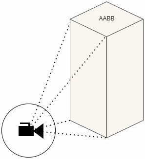
The compute pass that designates the LODs works something like this:

• We calculate and cache the AABB of all meshes vertex buffers in the scene (including vertex animated geometry).
• We estimate the solid angle of the view frustum on the camera unit sphere to determine which value constitutes as covering the entire screen. I do this by using great circles and Girard’s theorem. This calculation happens in local space, and can therefore be greatly simplified. I’ve added some comments explaining why it works:

// This calculates the solid angle of the near/far plane on the camera 
// hemisphere.
// 
// The frustum is symmetrical, so we only need to calculate a single angle.
// Because the solid angle stays the same regardless of view direction,
//  we assume tangent space.
// The frustum planes of the camera go through the camera position.
// This means they form great circles on the camera unit sphere.
// The angles between the frustum planes are given by their normals.
// Because of tangent space, the normal of the plane aligns with at least one
// axis. Two planes have an X and Z component, the other two a Y and Z.
// Since the angle is equal to the arccos of the dot product, 
// we can ignore the Y and X components (since they are multiplied with 0).
// This means that the only relevant component of the normal is Z.
// The Z component of the frustum plane itself then maps to the X component
// on a circle with the same rotation (cos(theta)).
// The Z component of the normal of that frustum plane then maps to the X
// component of the point rotated 90 degrees counter-clockwise (-sin(theta)).
// This means we can construct the normal of these planes
// by simply taking the -sin of their rotation angle.
// Because all planes are constructed in the same local space,
// we need to account for one of the planes starting with a 90 degree offset.
// This is equal to negating the -sin(theta) to be sin(theta).
let frustum_spherical_angle =
            (half_fov_radians.x.sin() * -half_fov_radians.y.sin()).acos();

// With the spherical angle of the frustum corner, Girard's Theorem
// can be applied to find the solid angle.
let screen_solid_angle = (4f32 * frustum_spherical_angle) - 2f32 * PI;

• We project each mesh’s AABB onto the unit sphere around the camera to get their solid angle. The solid angle is then divided by the view frustum solid angle, so that we get an estimation of how much of the screen could be covered by this object if we looked at it head-on.

‍

Aabb meshAabb = bnd.nodeBoundingBoxes.load<Aabb>(nodeHandle);

// World to local of the mesh instance.
float4x4 worldToLocal = inverse(bnd.worldTransforms.load(nodeHandle));

// The camera position, relative to the mesh in local space.
float3 cameraLocal = mul(float4(bnd.constants.cameraPosition, 1),
                                                    worldToLocal).xyz;

// Project the AABB onto the camera position. 
// Returns the solid angle in steradians.
float solidAngle = aabbIntegral(meshAabb.min, meshAabb.max, cameraLocal);

// We have a tweakable scalar to bias towards picking higher
// or lower quality LODs by pretending meshes are either closer or farther.
// Distance and solid angle of course scale by the inverse square law.
float lodDistanceScale = bnd.constants.lodDistanceScale;
float inverseSquareScalar = 1.0 / (lodDistanceScale * lodDistanceScale);
solidAngle *= inverseSquareScalar;

// Ratio of projected mesh to the solid angle of the screen.
float screenSize = solidAngle / bnd.constants.screenSolidAngle;

If interested, here’s a code sample of the aabbIntegral calculation. It takes the closest three AABB faces to the camera, and projects their four corners onto the camera unit sphere. It then applies Girard’s theorem to calculate the area of the spherical rectangle it forms.

// Calculate the integrated area of a polygon projected on a unit sphere,
// in steradians.
// The vertices are normalized directions from the center of the sphere
// to the corners of the polygon. This is based on Girard's theorem.
float quadIntegral(float3 verts[4]) {
  float sum = 0.0;

  // Calculate the normal for the plane on which each great circle lies.
  float3 normal1 = normalize(cross(verts[0], verts[1]));
  float3 normal2 = normalize(cross(verts[1], verts[2]));
  float3 normal3 = normalize(cross(verts[2], verts[3]));
  float3 normal4 = normalize(cross(verts[3], verts[0]));

  // According to Girard's theorem, the area of a polygon projected on a 
  // unit sphere is equal to the sum of its inner angles
  // minus (kPi * (N - 2)) where N is the number of vertices in the polygon.
  // Negate the 2nd component, because the normals are all pointing inwards.
  float dot0 = dot(normal1, -normal2);
  float dot1 = dot(normal2, -normal3);
  float dot2 = dot(normal3, -normal4);
  float dot3 = dot(normal4, -normal1);

  float sphericalExcess = acos(dot0) + acos(dot1) + acos(dot2) + acos(dot3);

  sphericalExcess -= 2.0 * kPi;

  return sphericalExcess;
}

// Returns the float closest to the base.
float minDistance(float base, float a, float b) {
  float diffA = abs(base - a);
  float diffB = abs(base - b);

  if (diffA > diffB) {
      return b;
  } else {
      return a;
  }
}

// Calculate the area of an AABB projected on the unit sphere around a
// position. The returned area is the solid angle expressed in steradians.
float aabbIntegral(float3 minBounds, float3 maxBounds, float3 eye) {
  // If eye lies in the bounding box, then the entire sphere is covered.
  if (all(eye >= minBounds) && all(eye <= maxBounds)) {
      return 4.0 * kPi;
  }

  // Calculate the edges of the visible 3 faces.
  float3 closest = float3(minDistance(eye.x, minBounds.x, maxBounds.x),
                          minDistance(eye.y, minBounds.y, maxBounds.y),
                          minDistance(eye.z, minBounds.z, maxBounds.z));

  float areaSum = 0.0;
  float3 verts[4];

  // Closest face on the x-axis.
  if (eye.x > maxBounds.x || eye.x < minBounds.x) {
      verts[0] = normalize(float3(closest.x, minBounds.y, minBounds.z) - eye);
      verts[1] = normalize(float3(closest.x, minBounds.y, maxBounds.z) - eye);
      verts[2] = normalize(float3(closest.x, maxBounds.y, maxBounds.z) - eye);
      verts[3] = normalize(float3(closest.x, maxBounds.y, minBounds.z) - eye);
      areaSum += quadIntegral(verts);
  }

  // Closest face on the y-axis.
  if (eye.y > maxBounds.y || eye.y < minBounds.y) {
      verts[0] = normalize(float3(minBounds.x, closest.y, minBounds.z) - eye);
      verts[1] = normalize(float3(minBounds.x, closest.y, maxBounds.z) - eye);
      verts[2] = normalize(float3(maxBounds.x, closest.y, maxBounds.z) - eye);
      verts[3] = normalize(float3(maxBounds.x, closest.y, minBounds.z) - eye);
      areaSum += quadIntegral(verts);
  }

  // Closest face on the z-axis.
  if (eye.z > maxBounds.z || eye.z < minBounds.z) {
      verts[0] = normalize(float3(minBounds.x, minBounds.y, closest.z) - eye);
      verts[1] = normalize(float3(minBounds.x, maxBounds.y, closest.z) - eye);
      verts[2] = normalize(float3(maxBounds.x, maxBounds.y, closest.z) - eye);
      verts[3] = normalize(float3(maxBounds.x, minBounds.y, closest.z) - eye);
      areaSum += quadIntegral(verts);
  }

  // Due to floating point precision problems, the area can be very slightly
  // negative when at 0-scale.
  return max(0.0, areaSum);
}

Runtime LOD Tweaking

As you may recall from the first chapter, we specify per mesh when we want the LODs to transition by providing a list of screen-sizes. If we specify 1, it implies we want to transition to this LOD only when the entire view is covered by that mesh. Likewise, 0 implies we want to use that LOD even if it is so tiny it’s not even visible. These values are calculated for us by the scene editing software we use. We upload them to the GPU so that our LOD designation shader can find the best matching LOD based on the AABB projection to view frustum projection ratio.

lod_activation_screen_sizes: [1.000000, 0.800000, 0.400000]

As you could see in the code samples earlier, there’s also a runtime scalar that we can use to fake objects being closer or further away using the inverse square law. Higher values will cause meshes to fall back to lower LODs more quickly, which is very useful when rendering at lower resolution devices such as phones.

float lodDistanceScale = bnd.constants.lodDistanceScale;
float inverseSquareScalar = 1.0 / (lodDistanceScale * lodDistanceScale);
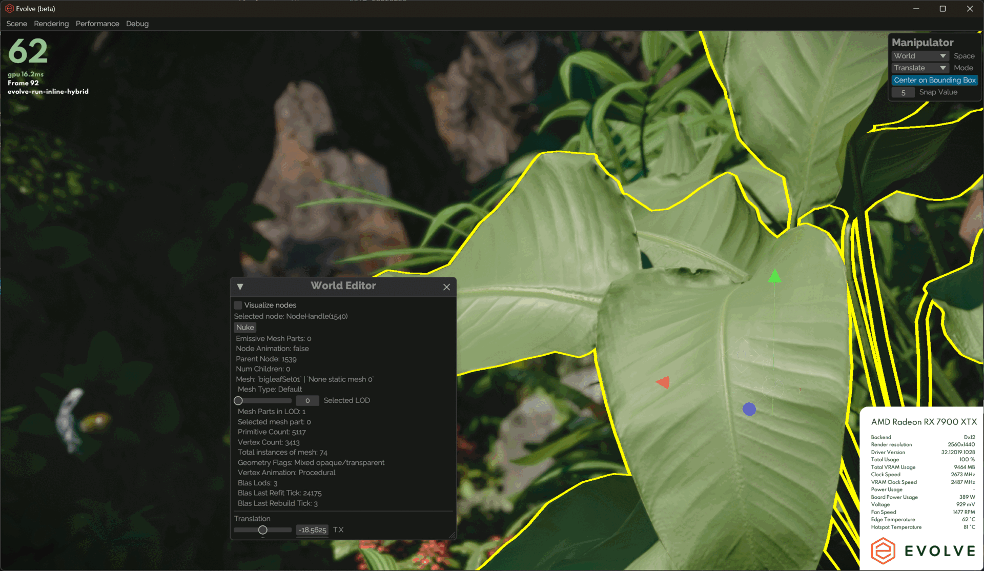
solidAngle *= inverseSquareScalar;

Other than that, I added some debug UI tools to allow us to manually lock in a specific LOD on the selected mesh.

Rasterization

The impact of having LODs on our rasterization passes is that we had to change to indirect drawing. As I mentioned before, sorting draw calls was a big bottleneck on the CPU, so this was a good opportunity to switch.

Now we simply dispatch a draw call for each mesh part (including the LODed ones), and set the actual draw count after we run our GPU based culling passes. We can then use the shader logic I showed before to access the geometry during drawing.

‍

Ray Tracing

Here I’ll explain how we do our TLAS and BLAS building each frame, and how it interacts with LODs. Because each LOD has unique geometry, we need a separate BLAS for each one.

1. Our compute shader to select a LOD for every mesh instance runs.
2. We go over all BLAS instances in the world, and swap their BLAS pointer with the one for the currently selected LOD. This happens in a compute shader as well.
3. We build the new TLAS from all the BLAS instances.

As you can see, this is problematic because we have to ensure all BLASes have been built or refitted before the TLAS build happens, but we don’t know which LODs have been picked on the CPU side. This could be solved by using indirect BLAS builds and refits, but there is no wide API support for this feature yet. We are stuck to doing CPU sided BLAS builds for now. So instead of doing a single build, we’ll now have to do one for each LOD as well.

We could add  a heuristic and read-back with  delay to make sure we can only pick BLASes that have been built so that we can reduce the amount of builds and refits per frame, but we chose not to solve this problem for the time being because of a few reasons:

• We know that 90% of our geometry is static. The BLAS only needs to be built once at startup, so we just do that for every LOD and call it a day. Startup time is a bit slower, but we can live with that.
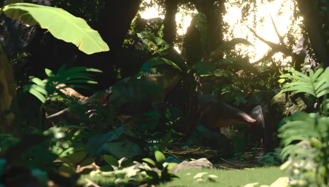
• For animated geometry, it would quickly become expensive to build a BLAS for each LOD level, but since vertex animated meshes (The player character and dinosaurs in the case of Evolve) are the focus of attention, usually we’d want them to be high quality anyways. We chose to not give them any LODs and instead rely on occlusion culling to reduce the raster performance impact when they are off-screen.
• We have many wind-animated plants in Evolve which use LODs. This may seem like a worst-case scenario at first, but we also use a wind pooling system so that we can reuse the same animated plant in more than one location. Because of this, most plants appear in many places and would likely have most LOD levels active at all times. In that case we would still have to rebuild all BLASes for the plants anyways, so there’s nothing to gain here.

We played around with having more than a single TLAS as well, so that we could have low level LODs in one for systems such as GI for cheaper tracing where the high frequency details don’t matter as much. In the end we abandoned this idea because the discrepancy in geometry caused severe darkening and artifacts in some areas. The cost of building an extra TLAS was also too large for any gains to be worth it on mobile hardware.

Results

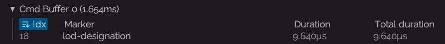
The overhead at runtime of this LOD system is very small. The only real additional cost is the LOD designation shader, which runs quite fast on an AMD RX 7900 XTX.

The BLAS refitting cost also isn’t terrible, despite refitting animated meshes and all their LODs each frame.

‍

‍

‍

Our VBuffer timings also show an improvement when we enable LODing.

Keep in mind that these timings were captured on a modern GPU. The difference on mobile devices is much larger and also has a much bigger impact. Most importantly, the system gives us a tool to tweak performance if the need arises. By far not all of our meshes use LODs, yet, and we could add more levels to the ones that do to further increase performance.

Final Thoughts

There are a few problems with our implementation, which I’ll briefly list here:

• No indirect BLAS refitting and rebuilding will likely form a new bottleneck in the future when we want to have animated LODs. Adding a slight delay in LOD selection and falling back to a “safe” one should be a good-enough solution until we get indirect refits and rebuilds.
• Shadow popping! A shadow can be right in front of the camera while its caster is not. If the LOD of the mesh switches, then you will see this happen. This depends a lot on the scene and light directions too, so we have been able to avoid the issue.
• We don’t have any in-engine solution to creating high quality LODs, and thus require an artist or external tool to do this work for us. Moving over to a Nanite-like system is definitely something that is interesting for the future.

At the end of the journey, we have a LODing system that works well without being intrusive in the rest of our workflow or rendering pipelines. The interface for binding meshes and accessing them on the GPU has not changed at all, so integration with existing systems was easy.

Most people don’t even know we have LODs, which means they work!

I hope this post has been informational. As always, feel free to reach out if you have any questions.

‍