Cooperative Vectors Introduction

A brief history

In 2021 we started investigating use cases for Neural Networks (NN) in our rendering engine. Our first successful attempt was with Neural Materials (NM).

Initially we only needed support for inference, since training of the NM was done "offline" in PyTorch. At the time, hardware accelerated inference was only supported through early vendor specific extensions on vulkan (Cooperative Matrix). Therefore, we built our own infrastructure for NN inference. This was built on top of our render graph, and fully in compute shaders (hlsl) without the use of any extension, to be able to deploy on all our target platforms and backends. One year down the line we saw impressive results from Neural Radiance Caching (NRC), which required runtime training of (mostly small, 16, 32 or 64 features wide) NNs. This led to the expansion of our framework to support inference and training pipelines.

While GPU’s had hardware dedicated to accelerate NN inference, there was not a way of accessing these features in shaders, especially cross-platform. For example, on desktop hardware we have different options per vendor: NVIDIA Tensor Cores, at the time, were only accessible through CUDA, and Intel's Xe Matrix Extensions (XMX) were vendor-specific, while AMD had Wave Matrix Multiply Accumulate (WMMA) instructions that use the "normal" shader cores.

As mentioned above, the Cooperative Matrix extension SPV_NV_cooperative_matrix, now elevated to KHR, was introduced as an abstraction for (tiled) matrix-to-matrix operations with the ability to access hardware accelleration, if present. This extension added new shader instructions to interpret buffers as matrices and to multiply them together. Similarly, DirectX added a very similar feature called WaveMatrix, initally intended for Shader Model (SM) 6.8, but then itnever realeased out of preview.

As a result of research on Neural Materials and Neural Texture Compression (NTC) by NVIDIA, they introduced a feature in Optix and a Vulkan extension: Cooperative Vector VK_NV_cooperative_vector. The solution proposed in the NTC paper compresses a set of textures for a material (like albedo, normal, roughness and metallic) into a NN and a learned texture-like representation. Both presented an interesting challenge: each material would have its own network, thus resulting in a situation where adjacent pixels on the screen might sample different textures, requiring an evaluation of a different network and therefore a different set of weights. This is not currently possible with Cooperative Matrix, which are meant for non-divergent work.

Similarly NM, have the same issue, where different pixels might require different sets of weights. The way we solved it in our inital implementation was to bucket queries to the same materials and run multiple dispachtes, one per material. This solution is not ideal, but works in practice, whilst being cumbersome and quite involved, ideally this should just be a branch in your shaders. Cooperative Vector solves this challenge by shifting interface from a matrix-matrix (in Cooperative Matrix) to a vector-matrix operation.

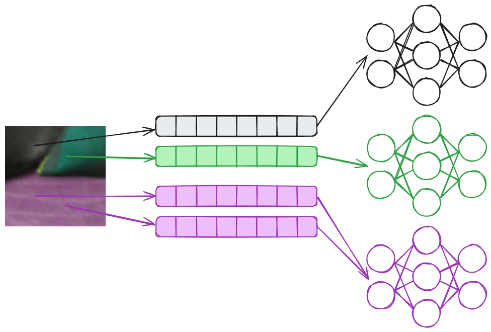
A simpler situation that still benefits from Cooperative Vector is NRC, illustrated in the image below. For NRC each pixel will contain different input parameters, like the normal (N), view direction (V), roughness (R), albedo (A) and specular f0 (S). Differently than NM, the input will be fed into the same network, which won’t require different weights/matrices. This scenario is the best case scenario, performance wise, for Cooperative Vectors, since this will be scheduled like a matrix-matrix multiplication by composing the input matrix by the input vectors.

What is a Cooperative Vector?

Let's clarify some terminology first: a cooperative vector, or long vector in Dx/HLSL, is the data structure itself. To avoid confusion, from now onwards, we will use long vector, when referring to the data structure. On the other hand, we will use Cooperative Vector to refer to the operations and hardware acceleration mechanisms that work with long vectors.

The "Cooperative" in Cooperative Vector refers to an implementation detail of the hardware acceleration, where individual vector-matrix multiply requests submitted by threads in a wave are combined into a matrix-matrix operation accelerated collectively for the wave. This name doesn't appear in HLSL code itself, just vector types and operations like vector-matrix multiplication as shown in the examples below.

So what are they exactly? Long vectors in HLSL are simply vector data structures that can be much longer than the usual 4 elements we've been used to in shaders. Nothing more, nothing less. They're a transparent data structure where the user can read and write individual elements via index, do operations on vectors like addition, multiplication, max (ReLU), etc.

From the looks of it, the registers for these vectors are directly stored as VGPRs (Vector General Purpose Registers), not in special registers even when hardware acceleration is available. From the perspective of a single lane (thread), the full long vector is stored in VGPR.

Thread / Execution Model

Now that we have an idea of what are Cooperative Vectors, where can they be used? At the moment, on both Vulkan and DirectX, they should be accessible in all shader stages, although we mostly use them in compute shaders . That being said, since the idea is to provide a way to support divergent data; in pixel and compute shaders we will have each pixel/thread hold its own long vector.

The most common way to implement it, and the most efficient way we found in practice, is to have each thread own its own long vector, although it is possible to store long vectors in shared memory. An important note: long vectors belong to the invocation (thread) they're declared in, or could be stored in shared memory, and don't require uniform control flow or fully occupied waves for functionality. On the other hand, uniform paths will enable driver fast paths for better performance, and features like Shader Execution Reordering (SER) could help with that.

The Matrices

Matrices come in two flavors:

Plain Layouts:

• Row Major
• Column Major

Optimal Layouts:

• MulOptimal (Inference)
• OuterProductOptimal (Training/Accumulation)

Accessibility in Shaders

Both Vulkan and DirectX provide interfaces that you can use to point to a memory address, like a buffer, and use it as a matrix.

For plain layouts (row/column major), we can address elements if we know the data type, matrix size, and layout. For optimal layouts, however, the memory addresses are completely opaque: we cannot do any read or write to a specific element, since the layout will be defined by the driver. Finally, the stride must be zero for optimal layouts, which prevents the user from accessing each element with indexing. This approach is an optimization similar to texture tiling.

So here's the key difference: long vectors and matrices in plain layouts are transparent, while matrices in optimal layout are opaque.

The idea is that the user will fill up their long vector manually in the shader. For example, within a wave each thread will hold a long vector with different UV coordinate, view direction, normal, etc. These long vectors are then multiplied by fixed matrices that should not be modified directly in that same shader.

‍

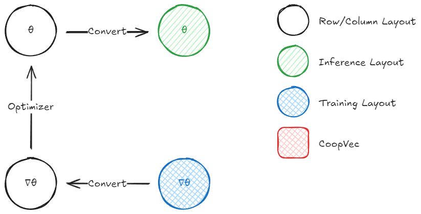
Inference and Training of a Network

One of the simplest NN, the Multi Layer Perceptron (MLP), is built as a sequence of linear layers and activations. Each layer computation can be performed by a single matrix-matrix or vector-matrix operation and addition of a bias and finally an activation, like ReLU.

Inference

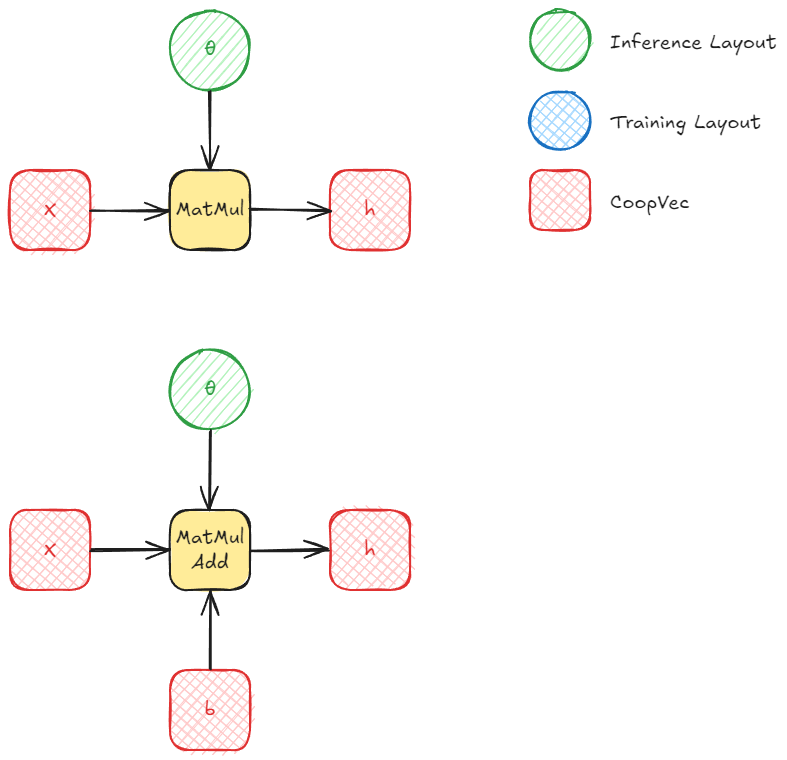
For inference, we can use either row/column layout or MulOptimal (inference optimal) for our weight matrices. Obviously, in the majority of cases, you'll want MulOptimal layout as it should be faster. In our experiments, there was a significant difference even for small matrices.

The way to fill out a MulOptimal matrix with the right data is to first write the data in row/column layout and then do a matrix conversion to optimal layout. Keep in mind that you need to query the destination size on the CPU before you allocate memory for the optimal layout matrix using ID3D12Device::GetLinearAlgebraMatrixConversionDestinationInfo. This is because the size is implementation-dependent (vendor, driver, etc.) and might require more memory than you would expect. Once this is queried and the data allocated, we can perform the conversion using ID3D12GraphicsCommandList::ConvertLinearAlgebraMatrix.

This conversion is essentially just a copy operation that rearranges the data into the hardware's preferred format.

Inference happens through MatMul (or MatrixVectorMul) or MatMulAdd. The second takes another long vector (in DX) or a matrix (in Vulkan) as input for the bias.

Training

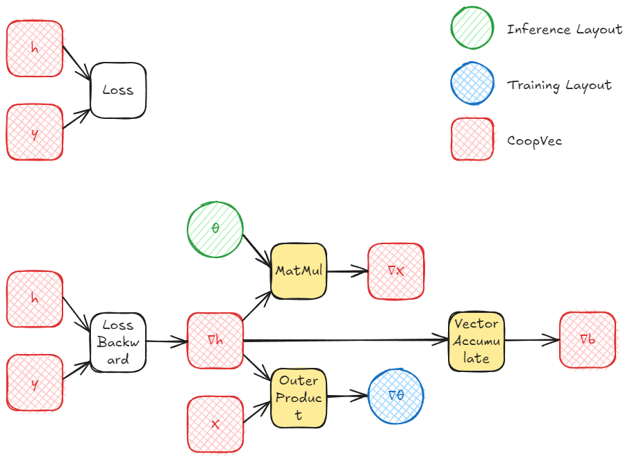
Training a single layer involves computing three gradients: the gradient with respect to the input (∇x), the gradient with respect to the weights (∇θ), and (optionally) the gradient with respect to the bias (∇b). After computing the gradient of the loss wrt the layer output h (∇h), we can propagate it back and we can compute these using cooperative vectors:

• Gradient wrt input (∇x): This requires multiplying the incoming gradient ∇h by the transposed weight matrix θ^T. Fortunately, the MatMul operation supports a transpose flag for MulOptimal (inference optimal) layouts, so we don't need to maintain a separate transposed copy of the weights.
• Gradient wrt weights (∇θ): This can be computed as an outer product between ∇h and the input x. This is where OuterProductAccumulate comes in, accumulating the gradient across a batch, where each row in the batch is a cooperative vector. This can also be computed as a matrix multiply, which could also be more efficient in some scenarios, but we'll be focusing on using all the features provided by cooperative vectors.
• Gradient wrt bias (∇b): If biases are present, their gradient is simply the accumulated ∇h across all samples, which can be done with cooperative vectors using VectorAccumulate, this is also a simple atomic addition.

The other optimal layout, OuterProductOptimal (training or outer product optimal), does not require a conversion from row/column to optimal per se, as this will usually be used for storing the gradients of the weights. On the other hand, if we use this layout, we would likely end up converting our gradients from OuterProductOptimal to row/column major at some point.

The OuterProductOptimal is used with the OuterProductAccumulate function (or coopVecOuterProductAccumulateNVin Vulkan). This takes two vectors and computes an outer product, which produces a matrix. This matrix is then accumulated into the target matrix, which MUST be in OuterProductOptimal layout. This operation is essentially a atomic addition/accumulation, where each element is atomically added to the corresponding element in the target matrix. Once this is done for all the batches in our training set, we can move on to copying the data with the conversion operation from OuterProductOptimal to a readable layout like row/column major.

What we're left to do is to add our gradient multiplied by a learning rate to the previous weights (in row/column). Note that this matrix-to-matrix operation is not possible using cooperative vector intrinsics at the moment, support for matrix-matrix operations is planned for future releases in DirectX, while Vulkan has cooperative matrix for this (though at the moment it seems to not be compatible with the optimal layouts, nor Cooperative/long vectors). For now, you'll need to handle this on the CPU or with regular shader code. After this is moved to the row/column major layout, we can convert it back to MulOptimal to use during inference.

And that is all!

Note that DirectX withdrew the Cooperative Vector proposal, and will instead land those features under a different name called linear algebra, which combines Cooperative Vector and Cooperative Matrix. All that was discussed in this article should stay relevant even after Linear Algebra, although with a slightly different api and names. On the other hand, Vulkan promoted Cooperative Matrix to KHR, while Cooperative Vector is still a NVIDIA only extension.