Intro to rendering of animated volumetric models in Breda

‍

All of these nodes have to be stored somewhere in a GPU friendly way, and thus we create a structure which we can upload to the GPU. This structure contains the following information:

All of these nodes have to be stored somewhere in a GPU friendly way, and thus we create a structure which we can upload to the GPU. This structure contains the following information:In this post, we’ll go over the basic building blocks of our real-time volumetric rendering process in the Breda graphics framework (developed at Traverse Research). This post is aimed at people experienced with general graphics algorithms like ray marching, writing shaders and some experience with bit manipulations. The following design goals were made very early in the development process and have guided the implementation so far:

— Loading of OpenVDB files
— Index space of 4096³
— Animation playback
— Voxels represent floating point data
— Small memory footprint to have enough space left over for other assets
— Needs to be ray traced in real time on an RTX 3070
— Multiscattering and emission support (not in this blog post)

Our data structure

Our data structure is a trimmed down version of the VDB data structure. We load VDB files using our custom parser called vdb-rs, and then load our structure into a format that includes only the features that we require. As with most VDB implementations we use the 5–4–3 structure which means that our top level node has an index space of 32³ (1<<5), our first internal node has an index space of 16³ (1<<4) and our last internal node has an index space of 8³ (1<<3). These combined result in an index space of 4096³ (1<<5+4+3). From now on, the different nodes will be referred to by their size, so Node5 is the top level node and Node3 the bottom level node. Below is a schematic of the structure:

These nodes are split up into 2 parts: a header, and a bitmask. Below is a description of one of these nodes, here the size of the bitmask is dependent on the level at which this node is located in the structure:

struct Node{
  child_pointer: u32,   // Points to the start of N_CHILDREN child nodes
  tile_value: f32,      // When the entire region is homogeneous
  min_value: f32,       // Minimum value of all nodes below it
  max_value: f32,       // Maximum value of all nodes below it
  mean_value: f32,      // Mean value of all nodes below it
  // Mask where every bit determines if one child node either 
  // contains data or not
  child_mask: [u32; N_CHILDREN / 32],
}

All of these nodes have to be stored somewhere in a GPU friendly way, and thus we create a structure which we can upload to the GPU. This structure contains the following information:

struct Volume{
  constants: Vec<VolumeConstants>,
  nodes5: Vec<Node5>,
  nodes4: Vec<Node4>,
  nodes3: Vec<Node3>,
  voxel_data: VoxelData,
}

As can be seen, we have vectors for the different node types. Additionally, we have a vector of constants, this contains information about the translation, scale and aabb of our volume. The reason why this is a vector is because these constants can be unique per animation frame. The last piece of the puzzle is our voxel data, which is stored in a large buffer containing the actual floating point data that the Node3 point to. This data is stored in bricks of 8³ voxels. Since this is by far the part of our data structure that consumes the most memory, our goal was to optimize it as much as possible. This is achieved by first changing the layout from a flat array (where each brick is stored as 8³ consecutive values) to a 3d texture layout, and then by storing the values in such a way that each 4 values in the z direction (of the brick) are stored as the RGBA components of our 3d texture. This allows us to run BC7 block compression and end up with 2 bits per voxel (floating point value). Below is a slice of the resulting texture:

Here each chunk of 8² pixels is half of an 8³ chunk, two of these slices make up the entire chunk. As can be seen, there are visible edges, corners and swirls in our data, even at this incredibly small scale.

Animations

As said earlier, we support animated volumes. These animations consist of sequences of VDB files which can be exported by programs like EmberGen or Houdini, or downloaded directly from JangaFX’s website (like we did in our examples below). You might have noticed that our Node5’s are also stored in a vector, but each of those nodes already has our desired index space of 4096³. So, instead, each of our animation frames has a unique Node5. This way, when switching to the next animation frame, we only have to change the starting point of our structure traversal.

‍

Structure sampling

Raymarching through volumetric space requires sampling the data structure a lot of times. This will likely be the hot-loop of our shader, so this has to be fast.

Sampling our structure requires checking if a child node is valid, and then follow the pointer down the tree. If the child node is *not* valid, we return the tile value, which indicates the value of all nodes beneath it. Once we are sure that the voxel exists, by checking the bit in our Node3, we sample our voxel data texture. Below is our code for doing that, note that all multiply, division and modulo operations are done using powers of 2, thus these are compiled to bit shifts and bitwise and operations.

float getVoxel(uint3 position) {
  // Assume we are in the aabb of the volume
  uint indexNode5 = computeIndexNode5(position);
  if (!getBitNode5(indexNode5, animationFrame)) {
    return tileValueNode5(animationFrame);
  }

  uint indexNode4 = computeIndexNode4(position);
  uint node5ChildPointer = getChildPointerNode5(animationFrame);
  uint node4Index = node5ChildPointer * kNode5Children + indexNode5;
  if (!getBitNode4(indexNode4, node4Index)) {
    return tileValueNode4(node4Index);
  }

  uint indexNode3 = computeIndexNode3(position);
  uint node4ChildPointer = getChildPointerNode4(node4Index);
  uint node3Index = node4ChildPointer * kNode4Children + indexNode4;
  if (!getBitNode3(indexNode3, node3Index)) {
    return tileValueNode3(node3Index);
  }

  uint node3ChildPointer = getChildPointerNode3(node3Index);

  // Our texture supports a maximum of kMaxBricksInDim^3 bricks, 
  // so wrap the indices to that region
  // node3ChildPointer to brick texture coordinates
  uint3 brickIndex;
  brickIndex.x = (node3ChildPointer % (kMaxBricksInDim));
  brickIndex.y = (node3ChildPointer / kMaxBricksInDim) % kMaxBricksInDim;
  brickIndex.z = node3ChildPointer / (kMaxBricksInDim * kMaxBricksInDim);
  brickIndex *= uint3(8, 8, 2); // multiplied by brick size, 
                                // each z texel stores 4 values

  // Offset inside brick
  uint3 texel;
  texel.x = position.x % 8;
  texel.y = position.y % 8;
  texel.z = (position.z >> 2) % 2;
  uint3 toSample = brickIndex | texel;

  // Position sample correctly in texture
  float4 chunkData = voxelData.load3D<float4>(toSample);

  // Grab correct z slice out of float4
  return chunkData[position.z & 3];
}

One function that needs further explaining is computeIndexNode. This is exactly the same as the internalOffset calculation in the OpenVDB paper. As input we get a position, then for every dimension we select only the bits that are relevant to the layer we are calculating the offset for. Then we place the selected bits into a single unsigned integer which is the the local index. Below is a code example which does this:

uint computeIndexNode5(uint3 position) {
  uint3 selected = (position & kNode5SLog) >> (kNode3Log + kNode4Log);
  selected.x <<= kNode5Log + kNode5Log;
  selected.y <<= kNode5Log;
  selected.z <<= 0;
  return selected.x | selected.y | selected.z;
}

There are a number of constants: kNode5SLog describes the log2 span of our Node5 (3+4+5=12) and the different kNodeXLog are simply the X values (so kNode5Log = 5).

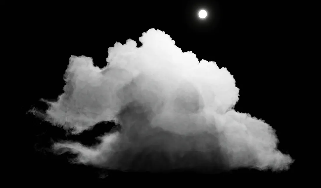
Simple rendering

To get some simple rendering going with our data structure, we can employ techniques commonly used in the game industry, as seen -in example- in 2.5D clouds rendering. For an in-depth overview of those methods, the challenges faced, and the solutions employed, we refer the reader to the extensive work available from Sébastien Hillaire as well as the various Nubis-related talks from Guerrilla Games.

Participating media is composed of particles which either scatter or absorb photons. Due to the extremely high amount of particles in a volume, this is all modelled through a statistical process in which the different kinds of particles are described by absorption (μₐ) and scattering (μₛ) coefficients.

A beam of light travelling through a differential volume element can undergo the following processes:
— Absorption
— Out-scattering
— In-scattering

The change of radiance travelling towards the ray direction must also account for emission, but we ignore it for this article to keep things contained.

We also focus on a single in-scattering event for the time being: the amount of light scattered back to the view as a result of the interaction between a light (in our case, the sun) and the media.

Absorption and out-scattering “remove” photons from the light ray travelling towards our eye, either because photons are absorbed or because they bounce off of the volume particles and away from the view. This process is a function of both the absorption and scattering coefficients, which -summed up- make up the extinction coefficient.
This can be represented with a single differential process, integrated along the ray direction, which gives us the transmittance along the ray as a function of the extinction coefficient. This is the Beer Lambert law.

In-scattering is a function of both the scattering coefficient and the phase function. The phase function describes the angular distribution of scattered rays for a volume, and is conceptually similar to a BRDF for surfaces.

We now have all the tools to understand the volume rendering equation

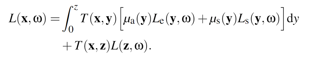
which tells us that the incoming radiance from point x towards the camera (ω) is the result of an integration process (with upper bound the surface point z) in which -at each step- the in-scattered radiance is modulated by the transmittance accumulated up to that step, and by the scattering coefficient at y. The exitant radiance at the surface z also contributes to the final output and is modulated by the total transmittance accumulated along the ray (the volume “translucency”).

We can approximate this integral as a Riemann sum, using ray marching.
Notice that transmittance is multiplicative along a ray

T(a→c) = T(a→b) · T(b→c)

which means that we can simply accumulate transmittance that way at each step of our integration.

With all that said, a simple (and naive) sampling routine would look like this:

for each pixel {

  TraceContext ctx = computePrimaryRay();

  float t0, t1;
  computeVolumeIntersectionBounds(out t0, out t1);

  // Variable needed for our final output
  float3 transmittance = 1.0;
  float3 scatteredLight = 0.0;

  // Results of our surface passes
  float3 reflectedRadiance = loadReflectedRadiance();

  // Better approach: start offset on view-aligned planes
  for each step with `stepSize` starting at t0 {

    // Compute scattering location
    float3 pos = ctx.origin + ctx.dir * (t0 + steppingDist);

    // Sample medium density at location
    float density = volume.sampleDensity(pos);

    if (density > 0.0) {
      // Calculate absorption, scattering and extinction coefficients
      VolumeCoefficients coeff = volume.getCoefficients(density);

      // Compute direct lighting
      float3 directLighting;
      {
        // Secondary volumetric trace towards the light
        float3 volumetricShadow = traceShadowRay(pos, dirToSun);

        // Compute phase function value
        float phaseFunction = volume.phaseFunctionEval(dot(dirToSun, -ctx.dir));

        directLighting = SUN_INTENSITY * phaseFunction * volumetricShadow;
      }

      float3 incomingLight = coeff.scattering * directLighting;

      float3 stepTransmittance = exp(-coeff.extinction * stepSize);

      // Improved integration for lower sample counts as presented by Sébastien Hillaire
      float3 integrationStep = (incomingLight - incomingLight * stepTransmittance) / coeff.extinction;
      scatteredLight += integrationStep * transmittance;

      // Accumulate transmittance
      transmittance *= stepTransmittance;
    }
  }

  float3 result = reflectedRadiance * transmittance + scatteredLight;
  writeOutput(result);
}

‍

‍

‍

Conclusion

This blog post went over the foundation of our real time volume renderer. Below is a demo of the renderer of a standalone volume. We can easily play back animations or manually change to the desired animation frame.

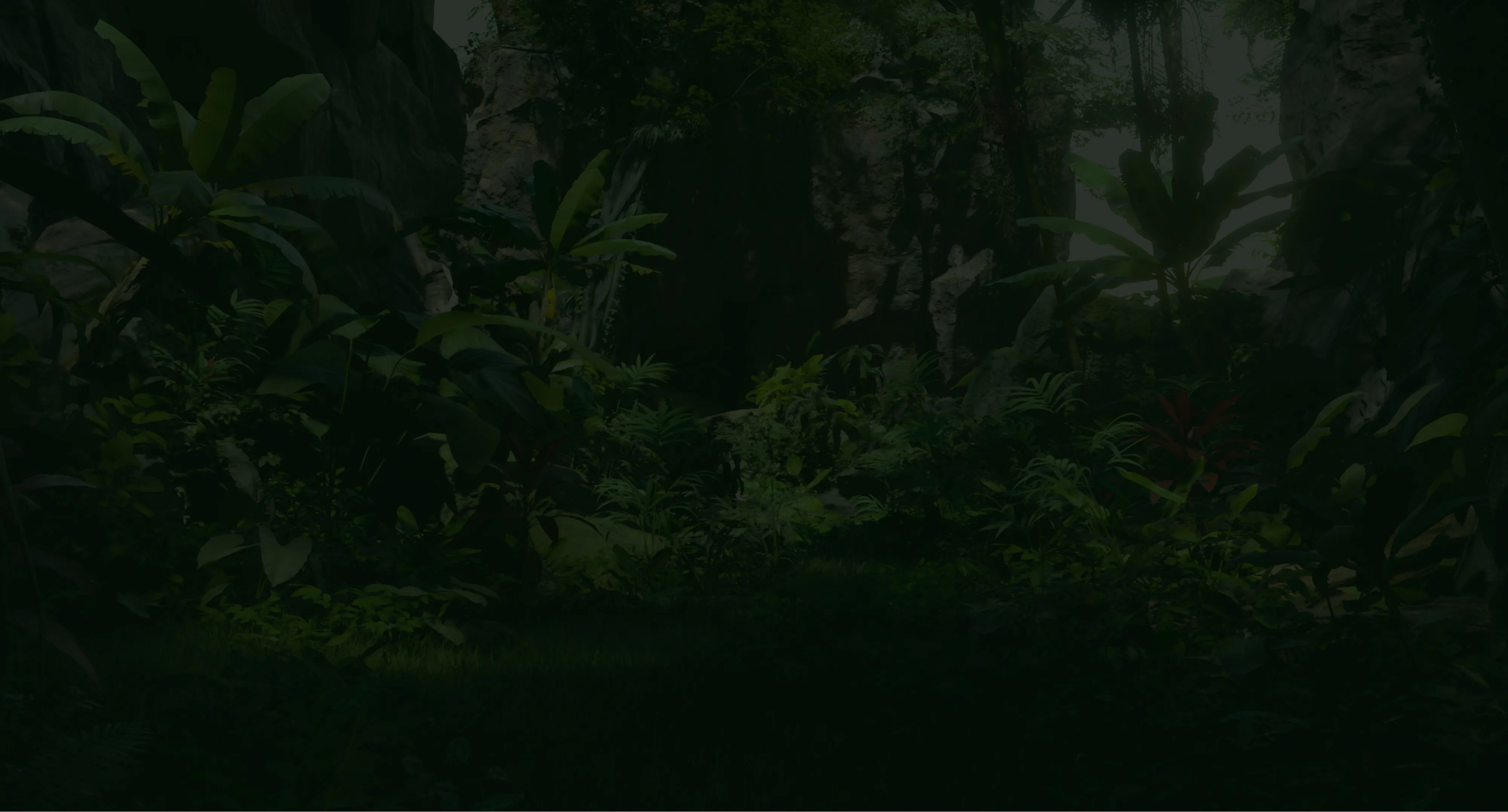
Below, we see a render from our Breda renderer. Here we placed a volumetric animation inside the Bistro scene.

This blog post was written by Emilio Laiso and Rosalie de Winther at Traverse Research. If you still have any questions, feel free to reach out on Twitter or directly to Traverse through our website.

This blog post was written in 2023 and recently migrated here.

‍

‍