Fast CDF generation on the GPU for light picking

In this blog post, I’ll take a deep dive into how we build our CDF for light sampling on the GPU at Traverse Research. I’ll give a quick rundown of what everything is, why you need it and finally how we made it run fast on the GPU.

The first few sections are an introduction to concepts that may not be clear to everyone, so feel free to skip ahead to the part where I dive into optimizing the GPU algorithm if you already have a good understanding of CDFs!

What is a CDF?

CDF stands for “cumulative distribution function”. In probability theory, it is a function that can tell you the probability that a random variable has taken on a certain value. This is done by summing the value of the probability density function (PDF) for each value that the random variable can assume.

The below diagram might make it a bit clearer if I’ve confused you up until this point: The red line is the value of the CDF for a random variable. The random variable can take on the values of A, B, C and D (X-axis), and the Y axis represents the value of the PDF for each of those values.

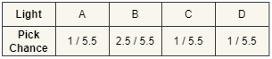
Personally I prefer to look at the CDF the way it is represented in code: an inclusive prefix sum array, where each element is the sum of the value of all elements that came before it (including its own value). The below diagram shows the PDF and CDF for the four values our random variable can assume in array form:

If you are interested in reading more about probability theory, then I recommend this blog post by Jacco Bikker.

Where and how are CDFs used?

With all that out of the way, you may be wondering why you would need a CDF. Well, it turns out that they are great when you want to stochastically select an element from a set proportional to its weight, and relative to the weight of all other elements in the set.

This is possible, because a useful property of CDFs is that you can invert them: rather than querying the CDF what value corresponds to a known element, you randomly generate a CDF value and find which element corresponds to it. That way you can select your samples with a priority for the important ones (the ones where the PDF gives a higher value).

A common scenario where this occurs is any algorithm that relies on monte carlo integration. If your dataset is too big to fully consider each iteration, then integrating over a few stochastic samples each cycle will eventually also converge to the correct result. By not taking random samples, but stochastically selecting based on weights you will converge to the right result faster. The stronger the relation between the importance of an element and its weight, the faster it will converge.

There are many algorithms where this applies, but for the rest of this blog I will be focusing on our use case: sampling lights in a real time ray tracer.

Light sampling algorithm

Let’s translate all that previous information to our use-case. We are running a real-time ray tracer with a scene that contains many lights. For every pixel, we want to know per light how much it contributes to the irradiance. In our actual implementation, we use monte carlo integration and we feed our selected light samples into a ReSTIR implementation, but for simplicity I will assume that we are only going to consider a single light per pixel, and that we are letting the image converge over time.

The algorithm is fairly simple, and works as follows:

1. For every pixel, pick a single light using the CDF.
2. Calculate the irradiance that the light contributes to the pixel, and divide it by the relative weight of the light.
3. Average the light contribution per pixel over many frames to get the correct result.

Step 1: Inverting the CDF
In an earlier section, I talked about inverting the CDF. This is exactly what we are going to do for step 1 of the algorithm! Let’s take the CDF from a previous example, and invert it. Pretend that A, B, C and D are the lights in our scene. Each light has a radiance, which we are going to use as its weight. This means lights that emit more energy will be stochastically selected by the CDF more often (since they are probably more important than weaker lights).

First we generate a random float between 0 and 1. Let’s say it landed on 0.75. In the image below, you can see we map this random float to the lights in the CDF and pick whichever one it landed on. In this case, that would be light C. Mapping the random float to the CDF is straightforward: multiply the random float with the sum of all light weights (which is the last element in the CDF) and then do a binary search in the array to find the element that contains the resulting value.

In this example, you would be multiplying 0.75 with 5.5, which gives you 4.125. Binary searching would yield you element C because it contains all values between 3.5 and 4.5.

Step 2: Calculating Irradiance
Cool, we have selected a light! We can now shade our pixel, but there’s still one important step: we must divide the resulting irradiance by the relative weight of our chosen light. Since we did not pick our lights uniformly, some lights will be overrepresented and others will seldom occur. Ignoring this problem would mean we are creating energy out of thin air, which is highly illegal. Fortunately for us, we can calculate the probability of having picked any one light by dividing its weight by the total weight sum of all lights.

We divide the shading result by the pick chance of our light. This will scale the light’s contribution up to compensate for all the lights that we did not pick this frame, proportional to how much the light contributes to the total light power in the scene. Light B would be scaled up less than light A, but B also gets picked more often. In the end this cancels out, and you are left with the same result that you would get from fully random light selection, but you needed less iterations to get to that result.

Step 3: Algorithm Integration & Conclusion
The result from one frame of this algorithm would be noisy, but if you average the results of a few frames it will quickly start to converge. For this scenario where we only have four lights, the algorithm does not make a large difference. But in modern path tracers, having hundreds of thousands of lights is a common scenario. That’s when this algorithm greatly reduces the complexity of shading.

CPU CDF Implementation

Now that we have all the theory out of the way, it’s time to actually build our CDF. On the CPU, a naive implementation of an inclusive prefix sum array is very simple:

  let light_weights = [1.0, 5.0, 2.5, 3.1, 1.0, 2.1];
    let mut cdf = vec![];

    let mut sum = 0f32;
    for light_weight in light_weights {
        sum += light_weight;
        cdf.push(sum);
    }

Naive CDF / prefix sum implementation on the CPU.

‍

After executing, the CDF would contain [1.0, 6.0, 8.5, 11.6, 12.6, 14.7].

The real downside to this implementation is that it is single-threaded, and building it takes O(N) time. If we had 16 elements we wanted to calculate the sum of, we would need to perform 15 additions in sequential order since the next addition always depends on the previous result.

We can then start using the CDF by stochastically selecting elements using some random number generation and a binary search like in the following code snippet:

/// Stochastically pick an element in the CDF and return its index.
/// The provided `rand` is a uniform random float with a value between 0 and 1.
fn binary_search_cdf(cdf: &[f32], rand: f32) -> usize {
    let max_value = cdf[cdf.len() - 1];
    let value_to_find = rand * max_value;

    let mut picked_entry = 0;
    let mut left_index = 0;
    let mut right_index = cdf.len() - 1;

    let max_searches = cdf.len().log2().ceil() + 1;

    for i in 0..max_searches {
        let center = (right_index + left_index) / 2;
        let higher = cdf[center];
        let mut lower = 0f32;
        if center != 0 {
            lower = cdf[center - 1];
        }

        if value_to_find < lower {
            right_index = center - 1;
        } else if value_to_find > higher {
            left_index = center + 1;
        } else {
            picked_entry = center;
            break;
        }
    }

    picked_entry
}

Binary search example on the CPU.

Parallel prefix sum

How do we make the build process faster than O(N)? Introducing: the parallel prefix sum! An algorithm that can calculate the prefix sum of an array of values using many threads at the same time, bringing the complexity down to O(log N). This algorithm requires a large amount of threads to be available at the same time, so it’s a perfect fit for the GPU.

The algorithm works by building a tree of local summed values in multiple passes. When the tree is completed, each element contains the sum of the elements below it. The top of the tree will contain the sum of all elements.

In our example, we will be building a binary tree from an array of 16 elements, so the algorithm needs 4 (log2(16)) passes. Each arrow represents a thread adding two values together and storing the result. If you count the arrows, you can see that we still need a total of 15 additions to get the sum of our 16 values. The difference is that we can run the additions largely in parallel! During the first pass, we perform 8 additions, but if we have 8 threads performing them at the same time, the total time taken is the same as doing one addition. Given that we have enough threads, the total runtime will be log2(N) additions where N is the amount of elements we want to sum.

Now that we have summed our values in tree format, we still need to flatten it into an array where each element contains the prefix sum at the index corresponding to the original weights array.

This requires one more pass where we launch a thread for each element in our weights array (16 threads in this case). Each thread remembers its element index, and that is where it will eventually write in the CDF array. We traverse the tree top-down, and our goal is to sum all values we find that are only composed of elements that have an index smaller than or equal to the current thread’s element index.

The logic looks as follows:

• Is the sum stored at the current tree node composed only of elements with an index smaller than or equal to the current thread’s element index? Then add the sum to our total. If the value already contains the current element index, terminate. We have found our prefix sum. If not, go down the right node of the parent node and repeat the algorithm.
• If the sum stored at the current tree node was composed of elements that lie to the right of our current thread’s element index, then we do not sum this value. Instead go down the node on the left and repeat the algorithm for that node.

The image above illustrates this logic for the thread that has been tasked with finding the prefix sum for the sixth element in our array.

1. It starts at the top of the tree, and realizes that the value there (27) also contains the sum of elements that came after index number six. It goes down the node on the left.
2. It checks if the value here (15) lies entirely to the left, but sees that it also contains elements seven and eight, which come after six. It goes down the tree on the left.
3. Finally! The sum here (7) is only composed of elements one, two, three and four. It adds 7 to our total sum. This sum does not yet contain our own element (six) so we go down the parents right node.
4. The value we find here (8) also sums elements that lie to the right of our current element. We go down the node on the left.
5. We find the sum of elements five and six (4). We add it to our total sum, which adds up to 11. Because the current node’s sum includes our current element (six) we can terminate the algorithm and write the prefix sum of index six: 11.

When all threads have finished executing, we are left with our prefix sum array. Knowing all this, it should be somewhat straightforward to implement the parallel prefix sum algorithm in a compute shader. There are however a few fun optimizations we can make!

‍

‍

‍

Single Pass Tree Builder

First of all, the algorithm requires multiple shader passes, one for each layer of the tree to be more precise. There needs to be an explicit synchronization between these passes because each layer reads from the previous one. Adding these execution barriers into our GPU timeline is slow, especially when we get near the top of the tree where we only need a few threads to do a few operations. Doing multiple compute passes also adds extra overhead.

Luckily, we can build the entire tree in a single compute pass by using a few HLSL synchronization tricks. This approach is based on a code snippet by Sebastian Aaltonen. I’ve made a greatly simplified version of our CDF tree building shader to showcase how it works:

// All threads in the same group will share the same atomic result.
groupshared uint atomic;

[numthreads(1, 1, 1)] void main(uint groupId: SV_GroupID, uint localThreadId: SV_GroupIndex) {

    // The tree buffer that we will be reading from and writing to.
    globallycoherent RWBuffer tree = [];
    
    // A buffer of atomics initialized to 0. 
    RWBuffer atomicsBuffer = [];

    for (int i = 0; i < treeDepth; ++i) {

        // The global thread ID is unique for all threads launched and corresponds to two elements in the tree layer below.
        uint globalThreadId = groupId + localThreadId;
        uint readOffset = treeOffsets[i];
        uint writeOffset = treeOffsets[i + 1];

        // This thread is only valid if the tree has one or two elements in the layer below that this thread should sum up.
        bool validThread = //..//;

        if (validThread) {
            // Sum the two elements in the previous layer and write them for the current layer.
            uint elementReadOffset = readOffset + (globalThreadId * 2);
            uint elementWriteOffset = readOffset + globalThreadId;
            tree[elementWriteOffset] = tree[elementReadOffset + 0] + tree[elementReadOffset + 1];
        }

        // One thread per thread group will update the groupshared atomic.
        // We halve the groupID so that two thread groups will end up writing to the same atomic.
        groupId /= 2;
        if (localThreadId == 0) {
            atomic = atomicsBuffer.interlockedAddUniform(atomicsOffsets[i] + sizeof(uint) * groupId, 1);
        }

        // Sync to ensure that the atomic for this thread group has been updated and will be visible for all threads in the group.
        AllMemoryBarrierWithGroupSync();

        // Two thread groups wrote to the same atomic, only the last one to write survives for the next tree layer.
        if (atomic < 1) {
            return;
        }

        // Sync to make sure that all threads within a group have finished reading the value of `atomic`.
        // This is needed because it will be modified again in the next iteration.
        GroupMemoryBarrierWithGroupSync();
    }
}

We start by launching enough thread groups to build the first layer of the tree: one thread for every 2 elements in our CDF array. Each thread will take the two elements from the previous tree layer, and then write a single element away to the next layer in the tree. We then kill off half our thread groups, since we only need to do half the operations in the next layer of our binary tree. Repeat this process until we have only a single thread that writes the top of the tree away.

The main issue with doing this is that every layer of the tree depends on the values in the previous having been written, so we must ensure that this writing has finished before we start reading.

The synchronization works because we keep re-using the same thread groups. The thread group that merges the two outputs from the previous layer, is the same thread group that wrote one of those values away in the first place. The other value was written by another thread group, but that group incremented the same atomic value as our current group. Since only the last group to write survives, we know that all data is there when we read it.

Only the first thread in each thread group updates the atomic in our atomics buffer, and writes the result away to group shared memory. This way all threads within that group can read the value after synchronizing.

You may have also noticed that I marked the tree buffer as “globallycoherent”. This is required because thread groups will be reading values written by other thread groups within the same shader invocation. That means that changes aren’t guaranteed to be written away to global memory from the local caches by the time we read again. The globallycoherent keyword ensures that any changes we make will be visible to other thread groups.

To make all this a bit more intuitive, here’s an example of the thread group lifetimes for a tree that is being built for an array containing 8 weights.

• We start with four thread groups, each consisting of a single thread for simplicity.
• Group 1 sums weight ‘2’ and ‘3’ and stores the result. It increments the atomic, and finds that it is the first to do so. It terminates.
• Group 0 sums weight `0` and `1` and stores the result. When incrementing the atomic, it reads back a value of 1, which means the other thread group it’s paired with has already finished executing. It survives because it knows it is the last group to finish.
• In the next iteration group 0 now reads the value it previously wrote, and the value group 1 wrote. From another part of the tree, group 3 is summing its own values and finishes executing first, so it terminates.
• Group 0 is now the last living group. During the last iteration of the tree building, it sums the value it wrote previously and the value written by group 3.

Optimal GPU usage

We now have a single compute shader invocation that can build our entire CDF tree, but we are not utilizing the GPU in a very efficient way. Having a single thread per thread group is far from optimal, so we should take a closer look at the hardware. It turns out that most modern GPUs schedule thread groups in smaller batches (warps or waves) of around 4 to 64 threads. If we make our thread groups the same size, we will be 100% utilizing the hardware’s thread lanes!

The next optimization involves wave intrinsics. GPUs execute shader code at exactly the same time for all threads within a wave. Special operations built into HLSL use this to allow you to read variables from other threads in your wave, since they are already loaded into memory anyways. We will be using the powerful “WavePrefixSum” intrinsic, which calculates the prefix sum for a variable for all threads in our wave with a lower index than the current thread.

// Most GPUs support 32 as wave size. After testing I found this to be the optimal solution on most hardware.
#define WAVE_SIZE 32
#define WAVE_SIZE_BASE uint(log2(WAVE_SIZE))

[numthreads(WAVE_SIZE, 1, 1)] void main(uint groupId: SV_GroupID, uint localThreadId: SV_GroupIndex) {
    for (int i = 0; i < treeDepth; ++i) {

        uint globalThreadId = (groupId << WAVE_SIZE_BASE) + localThreadId;
        bool validThread = globalThreadId < numActiveThreads;

        uint weight = 0;
        if (validThread) {
            weight = tree[treeOffsets[i] + globalThreadId];
        }

        // This wave intrinsic calculates the sum of the `weight` variable for all threads with a lower index in this thread group.
        uint sum = WavePrefixSum(weight) + weight;

        // The last thread in the group writes the summed value away.
        if (localThreadId == WAVE_SIZE - 1) {
            tree[treeOffsets[i + 1] + groupId] = sum;
        }

        //.. All that syncing and atomics stuff we did before ..//
    }
}

I’ve changed the previous code snippet a little bit to show how we would use this. Rather than one thread per group, we now have 32 (the most optimal number differs per GPU). Each thread loads a single element into memory, and the wave intrinsic calculates the sum incredibly fast. The last thread in our group then writes this sum away for the next level of the tree.

As you may have noticed, our tree is no longer base-2, but base-32. This is great because it means our tree isn’t as deep as it was before. We won’t need as much synchronization and we can process more elements in parallel. This does require some changes to the rest of our algorithm: the offsets for each tree layer will change, as well as the offsets for our atomics. Our thread groups are also no longer writing to an atomic in pairs of two, but in batches of 32. Each batch will be writing to the same atomic, and only the last one to write will survive. This makes sense: one out of every 32 thread groups survives, just like how we have 32 times fewer elements whenever we go up one level in our tree.

Similarly, the down-sweep pass that flattens the tree into an array will now also need to be updated to consider 32 children per node instead of just two.

Bonus optimization: since your wave size and tree base are powers of two, you can bit shift indices to the left and right instead of doing multiplication, division or modulo operations. This is a quite common scenario in this algorithm because you will often be calculating the offsets into the tree buffer for a given layer and thread index.

Layering multiple CDFs

That is pretty much the entire algorithm out of the way! I did however skip over one important detail of our ray tracing mesh light implementation. Up until this point I’ve been assuming that all lights are neatly laid out in a single array. Of course it can’t be that easy. In our actual implementation, any triangle of a mesh can be emissive, so when we pick a light we need to know the mesh and triangle index.

The solution here is to add more CDFs. We can build a prefix sum array for the number of emissive triangles in each mesh, and then inverse this CDF by flattening it into an array.

We can now use this flattened array as input for our light CDF tree shader. It will just involve a little bit of extra work for the threads that would normally only read the weights from the bottom level of the tree: they’ll have to load the triangle light using the indices in this buffer, and calculate that weight themselves (and store it for the bottom of the tree).

Floating point precision

While this algorithm is very fast, it does suffer from a few problems. The most important one is floating point precision. In a scene with a million lights, calculating the prefix sum means adding a lot of floats together. You end up with quite large numbers towards the end, which means lights with tiny weights may not actually change the sum at all anymore. They will thus never be considered. This problem can be mostly mitigated by sorting lights from low to high weight, but such a sorting pass would itself also take up time and may not be worth it.

‍

Conclusion & Timings

And that is how we stochastically select our lights at Traverse Research! In scenes with ~100.000 emissive triangles the whole process of breaking down our meshes and building the CDF for individual emissive triangles takes about 0.07 milliseconds on an AMD RX 6800 and 0.054 milliseconds on an Nvidia RTX 3080.

I hope this blog post was informative, and inspired you to use these techniques to speed up your own shaders. This was my first time writing a blog post, so feel free to send me some constructive feedback!

This blog post was written in 2022 and recently migrated here.